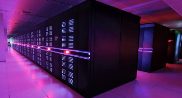
Dec 222014
 

Downturn

Tianhe-2 by Jack Dongarra

Tianhe-2


The semi-annual Top500 list shows a rather worrying trend for the 4th consecutive time in its last incarnation of Nov 2014. The list just hit its “lowest turnover rate in two decades.” The combined performance of the Top500 systems went from 274 Pflops to 309 Pflops in six months. The annual performance growth sits at ~23% at the moment, down from historic 90% per annum (measured between 1994-2008).

What this means is that there is practically no change in the Top500 most powerful computers in the world, and the trend is picking up speed in the wrong direction.
There are certainly cycles as technology and economies go through booms and busts, yet it seems there has never been this long a slowdown since 1993 when the list was first published.
There is only one new entry in the top-10 (in last place) with 3.58 Pflops from the US. To see the slope of the slowdown, here is a graph from the presentation.

There is reason to think the trend will reverse, eventually, but the best estimates point to the 2016-2018 period. That the trend can be traced to mid-2008 hints at the economic downturn as a cause. However, there is also reason to think competition has cooled off, or possibly technology is the bottleneck. This is support by the fact that a significant application area is government/military/classified, which aren’t nearly as sensitive to economic downturns as the scientific establishment. Technology is in the middle of a boom in terms of co-procs/embedded-proc as a new class of computers, so it’s hard to chalk this off as a technology bottleneck. If competition is to blame, it’s a mystery to me as to why this should be the case now, especially that US-China are more overtly in competition than ever before, at 46% and 12% entries respectively. Russia, with 2% of the Top500 entries, is at one of its lowest points in terms of relationship with Europe and the west since the cold war, and is implicated in a hot-war.

Supercomputing Performance Development - Copyright Top500.org

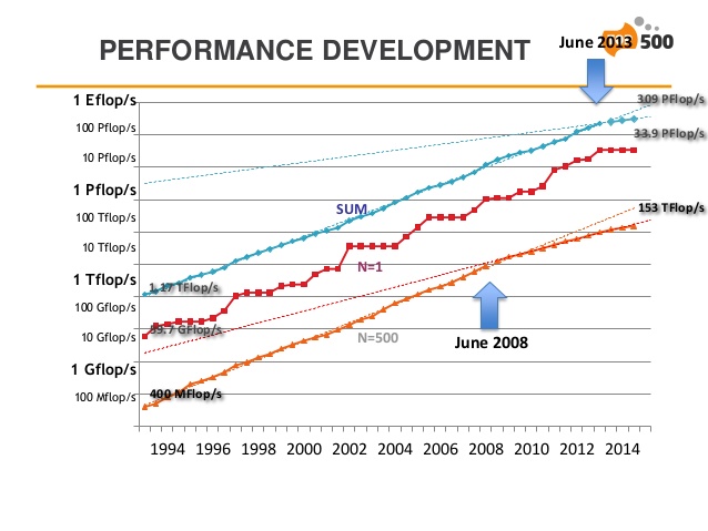
Supercomputing Performance Development and Stagnation

It should be mentioned that the US and Asia have lost a few percent points each in terms of entries since June last (Japan, the only exception, gained 2 entries) and Europe gained a few, surpassing China in raw power after being taken over two years ago. Perhaps the budgets and plans that reflect the political climate hasn’t yet materialized in terms of supercomputing power. It’s interesting to see how this will play out, as it’s a disturbing trend, one that has implications in terms of technology, science research, and a long history of healthy—and mischievous—competition between nations to simulate weather and destruction—both natural and man-made.

The presentation slides show the slowdown with all the glory and color of graphs and numbers.

Efficiency

The only relatively—good news is that the second most efficient system went from 3418 Mflops/Watt to a new record of 4272 Mflops/Watt since June last, improving on the top contender at 3459 Mflops/Watt by 23.5%.
In fact, there are five updated entries in the top-10 most efficient systems, four of which are new. Personally I find this exciting and encouraging, but without more raw power many applications can’t be improved further.

The Green500 list, which is similar to Top500 in that it tracks the world’s most power-efficient systems, as opposed to the most compute-capable ones, has more good news. The latest edition, which is published after Top500’s latest, lists two machines that are more power-efficient than the LX that holds the top entry in the Top500’s power-efficiency list. At 5271 Mflop/Watt, the L-CSC at the GSI Helmholtz Center in Germany improves on the LX by yet another 23.5%.
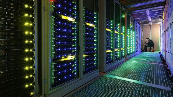
L-CSC at GSI, Copyright Thomas Ernsting from heise.de

L-CSC at GSI

To put this in perspective, the most efficient consumer GPUs hit 23 Gflops (for AMD) and 28 Glops (for Nvidia). However, these are the numbers for single-precision (32-bit) floating-point ops, not the “full-precision” required by the Linpack, which requires 64-bits or more. The double-precision GPU performance is 1/4th the single-precision, at best. Typically it’s 1/8th or less. For AMD the most efficient double-precision GPU will reach 5.5 Gflops and 7.2 Gflops for Nvidia, which aren’t the most efficient single-precision GPUs (GPUs are differentiated for different markets, so they don’t compete with themselves). Meaning that even the most efficient consumer GPUs hardly makes the cut on their own, without any overhead or even a motherboard and CPU. The L-CSC uses Intel Ivy-Bridge CPUs and AMD FirePro Workstation GPUs to achieve the efficiency record.

Exa-FLOPS

The above record performance if scaled to 1 Exaflops would require a mere 190 MW energy. While this is still significant, it is the closest we’ve come to the DARPA target of 67 MW (by 2020).
Whether the architecture of the L-CSC scales to Exaflops or not is a different matter altogether, but the energy efficiency question which hitherto has been the most formidable obstacle to reaching Exa-scale performance seems to be well within reach. Still, 67 MW is a rather optimistic target as it would require a 2.8x efficiency improvement over the current numbers. Nonetheless, in 2007, when plans for Exa-scale supercomputing was laid out, the technology of the day would require 3000 MW when scaled to Exa-flops. There has been, in effect, a net 15x efficiency improvement in the past 7 years (no doubt in major part due to co-proc technology).

On a related note, at least the US seems to have plans to pushing the envelope towards Exa-scale computing, according to a very recent announcement. The US gov. plans “to spend $325m on two new supercomputers, and a further $100m on technology development, to put the USA back on the road to Exascale computing.” The $100m is especially exciting news as it’s not going to a vendor for building or upgrading a supercomputer, rather it’s allocated for technology. Beyond that, this should give a decent push for the healthy competitive spirit to start rolling again.

How to Use a Million Cores?

There has been a significant research and interest in parallel algorithms and libraries in the past decade—in major part—precisely to address the issue of scalability. Most implementation of algorithms do not scale to tens or hundreds of cores (let alone thousands or millions,) even if in theory the algorithm itself is reasonably easy to parallelize. The world’s fastest single machine (by a margin of 2x from the next competitor,) the Chinese Tianhe-2, a.k.a. Milkyway-2, has 3.12 million cores to play with.

The main issue has to do with communication. But in the parallelizing algorithms, the major problem is even closer to raw computing—overheads. It seems that the biggest bottleneck to parallelizing efficiently on even the same socket is the overhead of partitioning, scatter, and gather. The last step of which typically is the killer.(Interesting presentation on scalability with HPX and more published papers here.) I’ve been following some of the libraries and compilers in the C++ world and HPX as well as TBB seem to be doing a very decent and promising job. HPX is especially promising and is well worth taking a look into as it’s C++ standards conformant and even has a good chance of getting some of its functionality into the standards body by 2017 (the next planned C++ standard voting meeting). In addition, it supports distributing across compute nodes. Like TBB, it’s OSS.

But the shorter answer is that these machines are designed for specific applications and typically have the software available, so there is a very good idea as to what hardware characteristics will deliver the best performance, both computational and power consumption. In addition, they run multiple parallel versions, or scenarios, concurrently that are independent of one another, which reduces scalability issues dramatically. This is actually a good thing for simulations as some, if not most, scenarios are discarded anyway, and the sooner one discovers their unfitness the better. I do not have the reference at hand at the moment, unfortunately, but I believe the record for scaling on the most cores was reached sometime back (circa 2013) with 1 million cores utilized towards solving a single problem, which is impressive by any measure.

Often the supercomputer is shared between users. The US Titan, the second fastest machine, has thousands of users and applications running on it. To that end the Lustre filesystem (based on ZFS) was practically created for it. With 40 PB storage and 1.4 TB/s throughput _on disk_, it’s not exactly a standard-issue I/O system. (This presentation on Lustre shows the performance achieved on Titan.) This means that Linpack numbers should be taken with a large grain of salt when comparing these behemoths.

Why Supercompute?

I’m perhaps as cynical as anyone about the utility of these beasts of a machine and I’ve pointed out the military use of these machines, which is unfortunate. However, I much rather have the testing of nuclear (and other WMD) done in virtual simulations on machines that push the state of the art and most likely trickle the technology down to civilian and commercial use, than to have them done by actually blowing up parts of our planet. Indeed, it was precisely the ban on nuclear arms testing that first pushed the tests literally underground (the French and the US are the best known examples of covertly resuming tests underground and in the oceans,) before ultimately going fully into simulation. As such, I’m not at all torn on my position when it comes to the use of supercomputers for military purposes, considering the aggressive nature of homo-sapiens (irony noted in the lack of wisdom when playing with WMDs) and the fact that there is beneficial side-effects to this alternative.

Now, if only we could run conflicts through simulations to avoid the shedding of blood, much like how territorial animals display their prowess by war screams and showing their fangs to avoid physical conflict, and walk away when the winner is obvious to both, I think the world would be a vastly better place. Alas, something tells me we do like getting physical for its own sake, often when there is absolutely nothing of significance to gain, and much too much to lose. Nobody said pride was a virtue without a cost.

Mar 102014
 

Cryptocurrency could’ve remained a theoretical exercise if it weren’t for the mysterious Satoshi Nakamoto, who was outed by Newsweek this week. The man allegedly behind Bitcoin had “a career shrouded in secrecy, having done classified work for major corporations and the U.S. military.” Whatever that means, and whether or not the face that has been linked with the name is the correct one, Bitcoin took a rather peculiar and big cat out of the bag.

Whatever you happen to think of the inventor, or inventors, of Bitcoin, which started a something of a revolution in economics similar to what the internet did to a couple of decades ago to information and publishing, and whatever you think of Bitcoin as an alternative currency, I hope to show that digital currency as a technology is separate and distinct from the economy and process of producing it. Let me state clearly from the outset that I don’t find digital currency as harmful as-such, rather that Bitcoin and the other breed of clones are extremely inefficient and wasteful. They could achieve, I argue, the same goals by being far more useful and valuable to society at large.

Bitcoins

We can agree that Bitcoin started something that will be hard to stop, if not impossible. This to me speaks of a demand for what Bitcoin has to offer. While some governments and media outlets tend to put the emphasis on illegal use of digital currencies, technically savvy users see it as efficient way of transferring funds, other users see it as a means to be independent from centralized power and a perfect candidate for a global currency. The efficiency of transferring digital currencies comes from lower transaction fees, but mostly because transferring them are done electronically and not physically. Anonymity, which is only partial, is also a highly sought trait in trade as it gives a sense of security and reduced risk, whether real or perceived.

The Other Side of the Coin

My objection to Bitcoin is not in the technology, nor its use. Put simply, everything has a cost, and the cost of the current crop of cryptocurrencies is rather high to society at large. I’m certainly not the first to notice this inefficiency and some tried to find ways to recoup the cost.

Those of us who have been planning on buying new video cards, a.k.a. GPU, are bitterly aware of the disproportionately high prices of the last generation of AMD cards. Back in December when these Radeon were in obvious shortage Litecoin mining was blamed. AMD improved its supplies of the highly demanded cards, but prices remain high. Eventually miners too had take note too.

There are many other uses to a GPU, besides the obvious mining and gaming, not least scientific and medical research, computer aided simulation, modeling and for finding drugs to cure deadly diseases among other promising and necessary projects. It is this latter group that is harmed by the high prices. And those were only the GPU-intensive projects. At this point CPUs are too slow to cost less in electricity than the potential coin value they mine, but of the projects that could use those CPU cycles are climate simulation and prediction, mind modeling, protein docking, and solar panel optimization to produce clean energy. And I’m leaving out many other HIV, cancer and other drug research projects.

To add insult to injury, not only is the high price of GPUs is reducing the potential number of participants on projects that have a chance of improving human life and prosperity, but they also don’t produce anything that benefits anyone other than the miner.

globe-home

But that’s not all. Cryptocurrency mining is a double whammy. The energy spent mining is energy wasted. On an individual level one might think there isn’t much difference between playing a game and mining. After all both use the same GPU and will consume the same electricity (per unit time,) which the owner is happy to pay for. However, unlike gaming, or more useful activities as mentioned above, mining has no entertainment value, doesn’t pay game developers that produce the games, doesn’t help us socialize as multiplayer games do, and do not have any hope of teaching us any skills that games might be argued to do. While I may lust over a multi-GPU gaming rig someone spent thousands to ramp up their frame-rate to run folding and similar projects on them when not playing, serious miners run farms of such rigs 24/7 to create money out of whatever their local power-station consumes to supply them with the juice that runs their cutting edge machines.

This isn’t unlike getting paid to produce soot. Or to pay power-stations to produce soot for you. Certainly we can do better and reverse the state of affair on its head: instead of burning away to mine coins, we can solve useful problems to mine coins. After all, digital coins are an arbitrary currency, and as I’ll show below, as long as we can secure it from attackers, what how many coins the work miner do produce and of what value a coin is, are completely up to us.

Before going further, let me state my point as clearly and tersely as I can: Regardless of how our personal ventures are paid for, there are very few investments that can rival the return on investment in scientific and medical research that will benefit the next generation, if not us directly, and we could still have digital currencies.

Economics 101

Traditional economics works by creating “value.” Suppose you have $100 million that you aren’t using at the moment. You can lend it to someone who has an idea for a project. They can do two types of things with it from an economics perspective: one possibility is to spend it all on hiring people to dig the biggest man-made ditch in the middle of nowhere, or, they can pay research centers that work on finding a new technology or a cure for a deadly disease. Of course there are countless other choices, and they don’t come in two colors either, they could use the money to build the next Google or Apple and create innovative products and millions of jobs. The point is that of all possible ventures and shades of black, there are those that go nowhere and do no good to anyone (except perhaps for feeding the workers and their families for the duration of the project, or until they commit suicide) and those that continue to serve most of society long after the project is over.

Any sound economic system should provide an incentive to the individual such that—to paraphrase Adam Smith—through self-interest participants inadvertently do more good to society by seeking to maximize personal gains. In my example above, the lender will be a fool for parting with his or her hard-earned money before first doing due diligence on how the funds will be spent. Yet, if everyone hoards their income and never lend out, society will need to constantly create more and more goods from some source that doesn’t require initial investment to match the growing demand. Clearly an unsustainable proposition. It is therefore in our interest to invest in fruitful projects. But, as I tried to show through my caricature of an example, the investment should pay us, both investors and society at large, more than it spends. Otherwise, eventually the economic cycle will slow down and come to a halt. This is exactly what happens in recession: investors lose confidence that they will get back their investments, so stop lending out.

If we could playback time and be in a position where we had a chance to invest in electronics in the ’50s and ’60s, to ultimately discover the transistor and then integrated circuits which made all of modern electronics, and not least computers, possible, such an investment would clearly have benefited investors and society. Similarly, if Dr. Jonas Salk had asked me for donations to buy equipment or even pay himself and his staff salary for his work on the polio vaccine, no awards will be given to me if instead I had decided to buy ice-cream to school children with the money, albeit arguably a reasonably good cause.

Granted, my examples are flawed: We don’t know in advance that Dr. Salk will succeed in producing vaccination for a disease that still stands without cure to-date and had infected as much as 350,000 children a year in 1988. In reality there would be many others working on similar vaccines and cures than just the one we know was successful post-factum. However, and this is my point, donating to any one of the researchers would be a much better long term investment to the very same children who received my free ice-cream.

Bitcoin Economics

To go back to digital currencies and economics, suppose I offer you 50c for smoking a cigarette. If you’re already a smoker, you might just ignore my joke or bother to take my money. If you’re not a smoker, I’m sure my offer will not convince you to start smoking. However if I were to make the offer indefinite, even a non-smoker might be tempted to do the math and find out that if they smoke 30 a day, they can make almost $5500 annually for the effort of a few minutes a day, and that can go even higher the more they smoke. I’m fairly certain that this offer, whether it comes from cigarette producers who are willing to pay for promotional purposes or otherwise, will have had a resonance as recent as a few decades ago when the harms of smoking were still unknown, if something very similar hasn’t been attempted already, which wouldn’t surprise me personally. In fact we should expect many people in poor conditions, who are either ignorant of the harms of smoking, or think it’s a lost cause to preserve their vanishing health anyway, might be tempted to take the offer.

Bitcoin does something very similar although in a different way. The offer is the following: participants in Bitcoin mining are rewarded for doing some work with a unique string of bits that they can use to trade with someone who’s willing to accept it in return of something of value, including goods, services, and of course cash. The inventor of Bitcoin made it easier to do said work than to counterfeit the “coins” (which are really just long numbers). (This is very important because if I were to offer you some product (or banknote) that people fake easily, you should immediately realize that you will have a hard time getting back what you paid for the original when everyone pays less for the fake.)

Unlike an employer, Bitcoin isn’t offering a work which has a purpose that is beyond our comprehension or need-to-know. The work Bitcoin is offering the reward for is completely arbitrary and, I argue, harmful to everyone, both participants and bystanders. Essentially, Bitcoin, and all cryptocurrencies to date, are offering a reward for finding a certain color and shaped grain of sand in the desert. They have designated sand hills to mine and the total number of said grains to be discovered. The value of the each grain is determined by the market and demand. And apparently there is a significant demand for them in markets that either want to be independent of the current monetary system, or, they like the efficiency of passing the grains around, once they find or buy them that is.

500 volunteers shoveling to move a dune in Lima from its original position.

500 volunteers shoveling to move a dune in Lima from its original position.

Once all the special grains have been discovered, the sand hills will be abandoned and all the trucks and shovels and all the work of digging, sieving and moving the sand will be forgotten. (This isn’t strictly accurate, as transaction fees will still make it lucrative for miners to continue validating and keeping a ledger of all transactions even when there are no new coins to discover.) But the energy and productivity lost to other more useful projects will be forever gone. What will linger along with the coins mined will be the long-term effects of burning so much electrical energy and building specialized hardware that, with the exception of general purpose GPUs and CPUs, have little or no use for much else than mining coins.

One response I got from a cryptocurrency aficionado was that it’s no different from mining for gold. It’s true that similarities between the two are abound, and I wholeheartedly agree that mining for gold can be similarly wasteful, but gold is a scarce metal that has numerous applications and uses beyond being used for monetary exchange and jewelry. Geology.com rightly calls it the most useful metal. Gold is used in the CPU and RAM that power your computer and in solar panels that produce electricity from sunlight. They are used in medicine and in industry and to make the reflective layer of early and high-end CDs. This is by no means an exhaustive list, but digital coins have nothing to offer in any of those applications anymore than they could be used in the successor of Hubble, the James Webb space telescope‘s mirror, or as a lubricant in space vehicles. Nor could they be used in surgical equipment.The monetary value of gold may be arbitrary from one point of view, but its value as a metal should never be underestimated.

In fairness, the shortcomings of Bitcoin I criticism are not not unexpected. After all it’s the first digital currency. Nonetheless, we should be aware of them and their real cost as more and more of the general public partake.

Mining: A Crash Course

As the the pool of miners explodes at an exponential rate, the majority is bound to be casual people who are no more interested in understanding how coins are really mined than the majority understands where and how money is created in the physical world. But here we are interested in going further.

Any currency, physical or digital, has some key properties to secure before having any chance of becoming sustainable as a legal tender. In the physical world control of over amounts in circulation, ownership and prevention of counterfeiting are done in centralized fashions. First, the central bank or an equivalent legal entity is given the monopoly right to print and issue banknotes. (There was a time when banknotes were handwritten IOUs that promised a payout to the holder issued by any “bank.” It was with the advent of permanent banknotes and central banks that this transformed into the current standardized single-currency per state form.) Second, transactions perform by an intermediary banks are managed by said banks such that one cannot double-spend or transfer funds from a fictive account and illegally increase their stash. These two institutions, central banks and commercial banks, are centralized. Centralization is an Achilles’ heel to any alternative currency because it can be controlled and shutdown easily, whether by legal means or by Denial of Service attacks. Distributed currencies on the other hand are immune to this, but at the expense of complexity.

The main issue in distributed systems is that because no single entity controls the ownership and total amount in circulation, there is distrust and the risk of hostile take-over by a rough party. To protect against such attacks, Bitcoin has a validation and voting mechanism built in. This is where the latency in validating transactions comes from. Before a transaction is complete, first a certain minimum number of other miners must confirm it. In Bitcoin the minimum number of confirmation is calculated to be six, which puts the difficulty of double-spending (i.e. spending the already transferred funds for a second time,) computationally unfeasible.

But how do you find coins in the first place? This is the interesting part as it is both intertwined with the confirmation process above as well as the mentioned problem of counterfeiting. Because of its distributed nature, the information that your bank holds secret must be available in public. Otherwise, where should it be if not in a central place, which we established isn’t desirable? Therefore, all transactions as well as wallet balances are also public information. What isn’t public is the identity of the wallet owners. But the network of transactions that they had committed and the wallets at each end of every transaction are also known. So one can trace the full history of all available coins and transactions and the balance of every single wallet are all public information. Now to create new coins, a miner has to do two things: First, it find the longest valid chain of transactions that it receives from other miners (remember that there are potential attackers who are sending out invalid transaction chains to essentially steal coins,) thus choosing the hardest chain to fake by an attacker (this is the confirmation stage). Second, they start finding a new block by simply finding a random number, such that: SHA256(last_hash + random) < last_hash

This formula a simplified, but the principle is preserved. The SHA256 is a function that takes a sting of bytes of arbitrary length and returns a fixed-length bytes (a long number really). The last_hash is also the result of an SHA256, and it is the hash generated by the last miner in the chain. Miners repeatedly call SHA256 on the new combination that they generate based on the random number (called nonce) and typically count the leading zeros of the resulting hash. If a certain number of zeros are found, then their work is complete and they send it to other miners in the network, which do exactly as we did when we received the block chain. Because we include the resulting hash and the random nonce that we used in the new block, they are able to repeat the same operation and check the result. The key here is in the difficulty in finding a random value and a resulting hash that when ran through SHA256 matches.

If someone else had beaten us to finding a nonce that fits the requirement, we will have to discard our work thus far on the block, check their block and once confirmed, we add their block to the chain and start the above process of mining on their block. Whoever finds a block by the above process is awarded a certain number of coins (typically 50 coins, which are halved at certain intervals). And because the blocks include all the information necessary to know who is who (by unique numbers that are as hard to forge as finding blocks,) and how much they have, all the information is shared in the pool and available to everyone. Thereby forging and faking becomes near impossible.

It’s worth mentioning that if an attacker controls more than half the mining nodes in the pool, they will be able to send out fake block chains that will allow them to double-spend their coins, because their voting power will basically be more than anyone else’s.

As it’s clear, the process of mining is arbitrary and the difficulty of producing coins is only to give strong guarantees that forging will be simply practically impossible. In fact, SHA256 is computed twice to make it even less likely that someone will find a trick or a way to reduce the amount of work they have to do to find a hash. This is like asking someone to throw a coin until they get, say, 500 heads in a row, but with the difference in that they can’t claim they have without actually having to do it, thanks to the cryptographic security of the SHA256 function.

A Better Digital Currency

Digital currencies certainly have their merits and we shouldn’t dismiss them out of hand. The current crop are the first and the technology is still young. They rely heavily on cryptography, whence they get their name, not least because cryptography is well-developed and understood. We know how to create secure messages that are very easy to create and validate but exceeding hard to break or fake. These are exactly the properties one want to have in any distributed monetary system. It is why banknotes are only minted by governments and they use state of the art printing technology to make counterfeiting expensive if not impossibly hard. But there is no reason why we should move sand hills that do little more than waste a lot of valuable resources all for the arbitrary coins that presumed to be in demand and therefore of value.

Proteins

There are other problems that are very hard to solve, but checking the answer is easy. These problems are known as NP-Hard and the more hardcore subset which are called NP-Complete. These are the hardest problems that exist, in computational terms. To give just one example of type of problems that could be used as a mining proof of work, optimizing the distance the electrical wires have to run in a computer, or the wires, piping etc in a city belong to a group of optimization problems that can’t be solved in a reasonable time except for the most trivial cases. Finding the shortest paths of wiring in a CPU will probably take longer than the universe exists even if all the computer in the world combined their power to solve it. Given a path, it’s trivial to add up the total length and see if it’s shorter than the shortest know or not. In currency system that is built around optimizing such a problem, those who have shorter paths will fetch more value than those with longer ones. There will be an economy, much like memorabilia collectors, where common items have a certain range of prices and highly-sought items that are known to exist have last-seen-price and then there are speculative items that is said to be worth a certain amount if it exists. When such a rare item (or path in our case) is put for sale, the market will decide its value. Alternatively, the first to improve on the previous record broadcasts their results and once validated by more people than any other solution, their block chain becomes dominant and all other blocks with inferior solutions are discarded. Finding the lowest energy protein folding secondary and tertiary structures is another similar problem.

There are many problems that are attention worthy and some of them are known to be very promising in deed. Digital currency could be the perfect catalyst to motivate people to donate more and more of their time and resources towards these goals while generating real value for them in digital coins. These aren’t new ideas by any means, and some have already made attempts at them. Some were pipe dreams, while others might have started in earnest.

Feb 152014
 

In the previous post we dived into Compression and Deduplication in ZFS. Here we’ll look at Deduplication in practice based on my experience.

To Dedup or Not to Dedup

Compression almost always offers a win-win situation. The overhead of compression is contained (not storage-wide) and except where there is heavy read/modify/write, it will not have unjustified overhead. It’s only when we have heavy writes on compressed datasets that we need to benchmark and decide which compression algorithm we should use, if any.

Deduplication is more demanding and a weightier decision to make. When there is no benefit from deduplication, the overhead will bring the system performance to a grinding halt. It is best to have a good idea of the data to be stored and do some research before enabling dedup by default (i.e. on the root). When the benefit from deduplication is minimal, the overhead will not only be in terms of higher memory usage, lower performance, but the DDT will be using disk space in the dozens, if not hundreds, of GBs. This means that there is a minimum dedup gain below which the overhead will simply negate the benefit, even if our hardware is powerful enough.

Regardless on the data, there are four scenarios that I can think of where deduplication makes sense. These are when:

    1. Duplicates are between multiple users.
    2. Duplicates are between multiple datasets.
    3. Duplicates are spread over millions of small files.
    4. Need copy-on-write functionality.

To see why the above make sense, let’s take a hypothetical case where we have one user and one dataset with thousands of GB-sized files. If we have duplicate files in this case, we can simply find them and hardlink duplicates. It should be clear that this will work perfectly, and it’s practical to frequently rediscover duplicates and hardlink them, except for the above four cases. That is, hardlinks don’t work across users (I’ll leave aside the issue of privacy and consider what happens when one user decides to modify a hardlinked file and inadvertently ends up modifying the other user’s version as well, since they are hardlinked,) they don’t work across datasets (i.e. filesystems) by definition (because inodes are only meaningful in a single filesystem) and hardlinking will be more complicated and a maintenance issue if our duplicate data is mostly a large number of small files. Finally, hardlinks simply means the filesystem is pointing multiple files to the same data. Modifying one will modify the other, which might not be desirable even in a single-user scenario, rather than create a new copy. ZFS dedup feature works using copy-on-write, so modifying a deduplicated block will force ZFS to copy it first before writing the modified data, thereby preserving the other previously-duplicate files to the one being modified.

If after ingesting data in a dedup=on dataset we decide to remove deduplication, we will need to create another dataset with dedup=off, and copy our data over (one can also use send/receive, which are beyond the scope of this write up see below). If you are in a situation where you have dedup enabled (at least on some of the datasets) but aren’t sure whether or not performance is suffering, there are a few tools I can suggest.

Monitoring Tools

zpool iostat [interval [count]] works very much like iostat except it is on the ZFS-pool level. I use zpool iostat 10 to see the IOPS and bandwidth on the pool averaged at 10 second periods.

Unfortunately, zpool iostat doesn’t include cache hits and misses, which are very important if we are interested in DDT thrashing. Fortunately, there is a python script (direct link) in the ZFS on Linux sources that does that.

arcstat.py [interval] dumps hit and miss statistics as well as ARC size and more (the columns are customizable, but the default should be sufficient). For those interested, arcstat uses raw numbers with some fields computed on the fly directly from /proc/spl/kstat/zfs/arcstats, which can be read and parsed as one wishes. Try cat /proc/spl/kstat/zfs/arcstats for example.

Here is a sample from my zpool showing the output of both tools at the same time while reading 95,000 files with an average of 240KB each. The dataset is dedup=verify and has a large percentage of duplicates in it:

               capacity     operations    bandwidth
pool        alloc   free   read  write   read  write
----------  -----  -----  -----  -----  -----  -----    ¦        time  read  miss  miss%  dmis  dm%  pmis  pm%  mmis  mm%  arcsz     c
tank        8.58T  7.67T    239     40  28.9M   101K    ¦    15:05:27  1.1K   238     21    14    1   224   97     7    2   3.0G  3.0G
tank        8.58T  7.67T    240     41  28.6M   103K    ¦    15:05:37  1.1K   236     21    16    1   220   98     8    3   3.0G  3.0G
tank        8.58T  7.67T    230     36  27.4M  91.7K    ¦    15:05:47  1.1K   229     21    17    2   212   97     8    3   3.0G  3.0G
tank        8.58T  7.67T    239     41  28.7M   102K    ¦    15:05:57  1.1K   234     20    15    1   218  100     7    3   3.0G  3.0G
tank        8.58T  7.67T    205     39  24.5M   101K    ¦    15:06:07  1.0K   215     21    17    2   198   99     5    2   3.0G  3.0G
tank        8.58T  7.67T    266     37  32.3M  97.3K    ¦    15:06:17  1.2K   255     21    15    1   240  100     5    1   3.0G  3.0G
tank        8.58T  7.67T    261     40  31.6M   104K    ¦    15:06:27  1.6K   272     16    13    0   259   99     7    1   3.0G  3.0G
tank        8.58T  7.67T    224     52  26.7M   239K    ¦    15:06:37  1.6K   229     14    16    1   213   96     8    1   3.0G  3.0G
tank        8.58T  7.67T    191     37  22.7M  93.0K    ¦    15:06:47  1.4K   200     14    17    1   183  100     8    2   3.0G  3.0G
tank        8.58T  7.67T    182     40  21.6M   103K    ¦    15:06:57  1.2K   180     15    15    1   165  100     7    2   3.0G  3.0G
tank        8.58T  7.67T    237     41  28.4M  98.9K    ¦    15:07:07  1.5K   241     15    13    1   227  100     7    1   3.0G  3.0G
tank        8.58T  7.67T    187     38  22.1M  96.1K    ¦    15:07:17  1.2K   183     14    16    1   166   99     7    2   3.0G  3.0G
tank        8.58T  7.67T    207     39  24.5M  99.6K    ¦    15:07:27  1.3K   201     15    18    1   182  100     9    2   3.0G  3.0G
tank        8.58T  7.67T    183     47  21.5M   227K    ¦    15:07:37  1.3K   199     15    18    1   181  100     9    2   3.0G  3.0G
tank        8.58T  7.67T    197     37  23.4M  95.4K    ¦    15:07:47  1.2K   183     15    16    1   167   97     7    2   3.0G  3.0G
tank        8.58T  7.67T    212     60  25.3M   370K    ¦    15:07:57  1.4K   210     14    16    1   193  100     8    1   3.0G  3.0G
tank        8.58T  7.67T    231     39  27.5M   104K    ¦    15:08:07  1.5K   223     15    17    1   206  100     8    1   3.0G  3.0G

The columns are as follows:

       pool : The zpool name
      alloc : Allocated raw bytes
       free : Free raw bytes
 (ops) read : Average read I/O per second
(ops) write : Average write I/O per second
  (bw) read : Average read bytes per second
 (bw) write : Average write bytes per second

       time : Time
       read : Total ARC accesses per second
       miss : ARC misses per second
      miss% : ARC miss percentage
       dmis : Demand Data misses per second
        dm% : Demand Data miss percentage
       pmis : Prefetch misses per second
        pm% : Prefetch miss percentage
       mmis : Metadata misses per second
        mm% : Metadata miss percentage
      arcsz : ARC Size
          c : ARC Target Size

Of important note is the IOPS relative to the bandwidth. Specifically, if the bandwidth divided by IOPS is <128KB, it means we are reading small files, which will affect performance compared to reading large files with sequential 128KB blocks. In other words, an average 25MB/s looks poor until we take into account that it is during reading 100s of small files (<128KB each) per second. For large files the average bandwidth is typically 10x higher.

ARC reads is rather high, betraying the fact that we are accessing deduplicated data. With ~15% ARC misses, we can assume that about 15% of our reads are wasted to ARC reads. Prefetching is virtually useless here (and if this were a typical usage, we should disable prefetching altogether, but for larger file reads prefetching pays dividends handsomely).

Another very important thing we learn from the above numbers is the low data and metadata misses. This is extremely important, arguably more important than ARC misses and DDT thrashing, as having high metadata miss-rate will translate in far higher latency in statting files and virtually any file operation, however trivial, will also suffer significantly. For that, it’s best to make sure the metadata cache is large enough for our storage.

During the above run my /etc/modprobe.d/zfs.conf had the following options:
options zfs zfs_arc_max=3221225472
options zfs zfs_arc_meta_limit=1610612736

We can see that the ARC size above is exactly at the max I set and I know from experience that the default ARC Meta limit of ~900MB gives poor performance on my data. For an 8GB RAM system, 3GB ARC size and 1.5GB ARC Meta size gives the most balanced performance across my dataset.

DDT Histogram

If you already have dedup enabled at all, a very handy command that shows deduplication statistics is zdb -DD . The result is extremely useful to understand the distribution of data and DDT overhead. Here are two examples from my pool taken months apart and with very different data loads.

#zdb -DD
DDT-sha256-zap-duplicate: 3965882 entries, size 895 on disk, 144 in core
DDT-sha256-zap-unique: 35231539 entries, size 910 on disk, 120 in core

DDT histogram (aggregated over all DDTs):

bucket              allocated                       referenced
______   ______________________________   ______________________________
refcnt   blocks   LSIZE   PSIZE   DSIZE   blocks   LSIZE   PSIZE   DSIZE
------   ------   -----   -----   -----   ------   -----   -----   -----
     1    33.6M   4.18T   4.09T   4.10T    33.6M   4.18T   4.09T   4.10T
     2    3.52M    431G    409G    412G    7.98M    976G    924G    931G
     4     250K   26.0G   23.0G   23.6G    1.20M    128G    113G    116G
     8    15.5K   1.07G    943M   1001M     143K   9.69G   8.29G   8.83G
    16    1.16K   46.0M   15.9M   23.2M    23.5K    855M    321M    470M
    32      337   7.45M   2.64M   4.86M    13.7K    285M    102M    195M
    64      127   1.20M    477K   1.33M    10.1K    104M   45.9M    116M
   128       65   1.38M   85.5K    567K    11.5K    258M   14.6M    100M
   256       22    154K   26.5K    184K    7.22K   45.5M   10.2M   61.1M
   512       11    133K   5.50K   87.9K    7.71K    101M   3.85M   61.6M
    1K        3   1.50K   1.50K   24.0K    4.42K   2.21M   2.21M   35.3M
    2K        2      1K      1K   16.0K    4.27K   2.14M   2.14M   34.1M
    4K        3   1.50K   1.50K   24.0K    12.8K   6.38M   6.38M    102M
    8K        2      1K      1K   16.0K    21.6K   10.8M   10.8M    173M
   16K        1    128K     512   7.99K    20.3K   2.54G   10.2M    162M
 Total    37.4M   4.62T   4.51T   4.52T    43.1M   5.27T   5.11T   5.13T

dedup = 1.13, compress = 1.03, copies = 1.00, dedup * compress / copies = 1.16

The first two lines give us footprint information. First we get the number of entries with at least 2 references (refcnt >= 2) and the size per entry on disk and in RAM. In my case 3.96m deduplicated entries are taking 3385MB on disk and 545MB in RAM. The second line represents the same information for unique entries (entries that are not benefiting from deduplication). I had 35.2m unique entries consuming 30575MB (29.9GB) on disk and 4032MB (3.9GB) in RAM. That’s a total of 33960MB (33.2GB) on disk and 4486MB (4.4GB) in RAM in 39.2m entries, for the benefit of saving 12-13% of 5.13TB of data, or a little over 600GB.

This is not that bad, but it’s not great either, considering the footprint of the DDT, the benefit of saving 12-13% comes at a high cost. Notice that compression is independent of dedup gains and so I’m not accounting for it. Although it’s nice to see the overall gains from dedup and compression combined. We’ll get to copies in a bit.

The histogram shows the number of references per block size. For example, the second to last line shows that there are 16-32 thousand references to a single block that has a logical size (LSIZE) of 128KB taking 512 bytes physically (PSIZE,) implying that this is a highly compressed block in addition to being highly redundant on disk. I’m assuming DSIZE is the disk size, meaning the actual bytes used in the array, including parity and overhead, for this block. For this particular entry there are in fact 20.3 thousand references with a total logical size of 2.54GB but compressed they collectively weigh at only 10.2MB, however, they seem to be taking 162MB of actual disk real estate (which is great, considering without dedup and compression they’d consume 2.54GB + parity and overhead).

Powered by this valuable information, I set out to reorganize my data. The following is the result after a partial restructuring. There is certainly more room for optimization, but let’s use this snapshot for comparison.

#zdb -DD
DDT-sha256-zap-duplicate: 1382250 entries, size 2585 on disk, 417 in core
DDT-sha256-zap-unique: 11349202 entries, size 2826 on disk, 375 in core

DDT histogram (aggregated over all DDTs):

bucket              allocated                       referenced
______   ______________________________   ______________________________
refcnt   blocks   LSIZE   PSIZE   DSIZE   blocks   LSIZE   PSIZE   DSIZE
------   ------   -----   -----   -----   ------   -----   -----   -----
     1    10.8M   1.33T   1.27T   1.27T    10.8M   1.33T   1.27T   1.27T
     2    1.07M    124G    108G    110G    2.50M    292G    253G    258G
     4     206K   22.5G   11.4G   12.4G    1021K    112G   50.9G   56.1G
     8    18.7K    883M    529M    634M     177K   9.37G   5.47G   6.43G
    16    31.0K   3.80G   1.67G   1.81G     587K   71.8G   31.9G   34.5G
    32      976   93.7M   41.6M   46.6M    42.2K   4.09G   1.80G   2.02G
    64      208   13.0M   5.30M   6.45M    17.0K   1.04G    433M    531M
   128       64   2.94M   1.30M   1.73M    11.1K    487M    209M    286M
   256       20    280K     25K    168K    7.17K   81.0M   10.0M   60.7M
   512        8    132K      4K   63.9K    5.55K   80.5M   2.77M   44.4M
    1K        1     512     512   7.99K    1.05K    536K    536K   8.36M
    2K        4      2K      2K   32.0K    11.9K   5.93M   5.93M   94.8M
    4K        3   1.50K   1.50K   24.0K    19.8K   9.89M   9.89M    158M
 Total    12.1M   1.47T   1.39T   1.40T    15.2M   1.81T   1.60T   1.62T

dedup = 1.16, compress = 1.13, copies = 1.01, dedup * compress / copies = 1.29

A quick glance at the numbers and we see major differences. First and foremost the DDT contains only 12.7m entries (down from 39.2m above,) while the dedup ratio is up at 15-16% (a net gain of ~3%). Compression is way up at 13% from 3% with a slight overhead of extra copies at 1%. The extra copies showed up when I manually “dedpulicated” identical files by hard-linking them. Normally copies “are in addition to any redundancy provided by the pool, for example, mirroring or RAID-Z. The copies are stored on different disks, if possible. The space used by multiple copies is charged to the associated file and dataset, changing the used property and counting against quotas and reservations.” according to the ZFS man page, but I’m not entirely clear as why they showed when I hard linked large files and not, say, when I already had highly-redundant files which could benefit from extra redundancy in case of an unrecoverable corruption.

What really counts in the above numbers is the relative effectiveness of deduplication. That is, the higher the dedup percentage, the lower the overhead of unique blocks becomes. It’s true that I reduced the number of duplicate blocks, but that’s mostly because I either deleted duplicate entries or I hardlinked them. So they weren’t really beneficial to me. Meanwhile, I reduced the number of unique entries substantially, increasing the utility of deduplication. This means the overhead, which is now far lower than it used to be, is being utilized better than before. This gives me an overall net gain that could be quantified by the dedup * compress / copies formula, which went from 16% to 29%, which is almost double.

I still have more work to do in optimizing my data and deduplicated datasets. Ideally, we should only have dedup enabled on datasets that either gain at least 20% from deduplication (although some would put that number far higher) or the unique blocks are potential duplicate entries pending future ingestion. Unique data that is deemed to remain unique has no place in deduplicated datasets and should be moved into a separate dataset with dedup=off. Similarly, duplicate that that is best manually deduplicated by hardlinks, or duplicates deleted, should be done so to reduce undue overhead and waste.

Undeduplication

Once we decide that a dataset is not benefiting from deduplication (typically by finding duplicates across the full zpool or by doing other statistical analyses,) we can set dedup=off on the dataset. However this will not remove blocks from the DDT until and unless they are re-written. A fast and easy method is to use send and receive commands.

First, we need to either rename the dataset or create a new one with a different name (and rename after we destroy the first).

#Rename old dataset out of the way.
zfs rename tank/data tank/data_old

#Take a recursive snapshot which is necessary for zfs send.
zfs snapshot -r tank/data_old@head

#Now let's create the new dataset without dedup.
zfs create -o dedup=off -o compression=gzip-9 tank/data

#And let's copy our data in its new home, which will not be included in the DDT.
zfs send -R tank/data_old@head | zfs recv tank/data

#Remove the snapshot from the new dataset.
zfs destroy tank/data@head

#Validate by comparing the data to be identical between data and data_old.

#After validating everything, destroy the source.
#zfs destroy -r tank/data_old

The end result of the above is to remove a dataset form the DDT.

Note that a -F on recv will force it, which will not fail if data has some data! This is useful if we need to start all over after moving some data into the new dataset. There is a -d and -e options, which are useful for recreating the tree structure of the source. These are typically needed when datasets move between pools. To see the target tree with a dry run, add -nv to recv. Note that the target dataset will be locked during the receive and will show empty using ls. The output of send can be redirected to a file or piped into gzip for backup.

Hope you found this helpful. Feel free to share your thoughts and experience in the comments.

Jan 262014
 

In the previous post we looked at performance and benchmark statistics on a home NAS/HTPC with ZFS on Linux. Here we’ll take a deeper dive into some of the more interesting features of ZFS–Compression and Deduplication.


When I set out to build a NAS I aimed for the lowest cost with the best utility. My primary goal was to move all my precious (and the less-than-rare) files in a redundant storage that is accessible, manageable and low-cost, but reliable. The idea of extending it to HTPC came to me after comparing prices of commercial home/small-biz NAS solutions with the cost of the bare components. One can do so much more with a generic Linux box than a specialized black-box. However I wasn’t willing to pay a premium to turn what started out as NAS into a general purpose rig; It had to be low-profile.

ZFS offers enterprise-level features and performance at the cost of maintaining it. Never underestimate the overhead of maintenance though. The biggest issue I’ve had to face with ZFS on Linux was that of memory starvation. I had read that ZFS has less than humble memory requirements and it could always put more of it to good use. Recommendations of 1-2GB / TB of storage floats on the web. However I ended up supplying it with only 8GB for 18TB of storage to be shared with the OS and other applications. The experience is worth sharing, especially the lessons learnt, which should prove worthwhile for others with similar plans to mine. But first, we need to take a look at some of the internals of ZFS.

Compression vs Deduplication

Both compression and deduplication are designed to reduce disk space usage as much as possible. One should keep in mind that these features don’t come for free and there are caveat to be aware about. First and most important point to keep in mind before deciding which features to enable is that deduplication happens on the zpool level. The pool is at the volume management layer and dedup works on the block-level, away from any file structures. The filesystem dataset sits atop the zpool and that’s where compression works, before deduplication is done. When enabled, zfs compresses each block using the chosen compression algorithm and writes to the pool. While writing, the zpool compares the checksum of the incoming block with existing block checksums, and, if a match is found, the matching block’s reference count is incremented, the block reference ID passed back to the filesystem and no data is written to disk (expect the reference count increment in the deduplication table).

Neither dedup nor compression work retroactively. So a change in either setting will not propagate to existing data. When new data is written, or old data read/modified/written, the new settings will take effect. Due to the fact that compressed block data depends on the compression algorithm (and level,) identical blocks compressed with different compression algorithms virtually certainly will not match as identical (although their uncompressed bytes match). This is only an issue when the pool has identical duplicate data in different datasets with different compression algorithms or level. Datasets that have similar data that can benefit from deduplication will lose that opportunity if they utilize different compression settings. Changing the compression setting of a dataset should be done when one is fairly confident that the gains will outdo any loss of dedup opportunities with other datasets with a different compression setting.

Compression

The overhead of compression is very much contained and bounded in that the hit is taken for each block at the time of reading and writing to that block and that block alone. Compression will require no extra disk space beyond the compressed file bytes and the memory overhead is typically negligible and of fixed size (because the block size is also fixed). Do note that a block will be written uncompressed if after compression there is no saving of at least 12.5% (1/8th) of the block size. That is, for a 128KB block, if compression doesn’t save at least 16KB, the block will be written uncompressed. Future reads will not have any decompression overhead of course, but re-writing said block will go through the same compression cycle to decide whether or not to write the compressed version. Notice that the compression algorithm and level is stored with each block, so changing these values on the dataset does not affect existing data, but only apply to future modify and writes. Naturally when a block is written uncompressed the metadata of the block will mark it as uncompressed. This means that having uncompressible media files on a compressed dataset will only incur the overhead of compressing at ingestion time and, in virtually all cases, the uncompressed data will be written to disk, and no overhead when reading (I read the code to be sure). Where compression could make a net gain of 12.5% or more, those blocks will be written compressed and it’d only be fair to pay the penalty of decompression for them and them alone when reading.

By default, lz4 compression could be used, unless we know we will store incompressible data, such as already compressed video or audio files, that will not be write-once read-many (WORM). If files will be modified heavily, we have to make a very educated decisions (read: experiment/research before you commit). While for highly compressible data (such as source code, databases, XML dumps etc.) gzip will do much better than lz4, it will also have a much higher CPU cost, and for those who care about it, latency. On the other hand, if you use gzip, it wouldn’t matter much whether you use gzip-1 or gzip-9 (relatively speaking to lz4, that is). My preference is to default to gzip-7 for the root of the pool and either choose no compression (very rarely) or choose gzip-9 for all WORM data.

Deduplication

Unlike compression, Deduplication has to keep track of all blocks in the pool (that belong to datasets with dedup=on). The number of blocks will be at least as large as the number of files, in the rare case that each file is less than or equal to a single block size. In practice, the number of blocks will be orders of magnitude larger that the number of files. Each block will therefore have both a disk, memory and cpu overheads. All three resources will increase the more the blocks we have. On disk the dedup tables (DDT) are stored to survive reboots, which are loaded to memory to maximize the performance of finding matches when writing files, which will require more processing the more the block checksums there are to compare against. Of the three the most worrisome is the memory overhead. On disk a few extra gigabytes will not be noticeable and searching even trillions of checksums should take microseconds at worse. It’s the memory needed to hold said trillions of checksums to perform fast comparisons is the problem. It is recommended to have 1-2 GB of RAM per TB of disk for good performance. Interestingly, the more duplicate blocks in the pool, the smaller the memory requirement per entry will be. This is because the DDT stores the unique block checksums that are written to disk, which is less than or equal to the total number of blocks. So a pool that doesn’t benefit from deduplication will be wasting more resources than one that is benefiting handsomely. As such, if we do not expect a significant gain from deduplication, the overhead will not be justified and should be avoided by disabling it.

Deduplication works on the block level. It computes a checksum per block and looks up the checksums in a deduplication table (DDT) to find duplicates. The default checksum is sha256. Although sha256 is a cryptographic hash (meaning it’s designed to have great avalanche characteristics and be exceedingly difficult to synthesis,) there is still a negligible chance that two different data blocks might hash to the same value. For the paranoid, ZFS dedup supports verification by byte comparison when checksums match and before assuming the blocks to be identical (and discarding one for the other). However, and as dedup author Jeff Bonwick has pointed out, the chance that sha256 will have a collision is less than that of an undetected ECC memory error, although the actual error rate by chance is far higher than he calculates due to the birthday paradox. Because this miscalculation is parroted elsewhere, it might be worthwhile to point out why it’s wrong.

Checksums, Collision and the Birthday Paradox

Sha256 has 256 bits, and while it’s true that a single random bit flip will have a chance of 1 in 2^256 to match the same hash as another block, in reality we do not have just two hash values but millions. We are worried that a corrupted block will change the hash of that block such that it matches any other block’s hash, and of course all blocks are subject to the same possibility of corruption. To go back to the birthday paradox (which asks about the minimum number of people in a room so there’d be at least 50% chance that any two share the same birthday,) the question here isn’t about the chance that another person shares your birthday, rather that anyone shares any other’s birthday (or in this case hash-value). The chances are obviously higher than just 1 in 2^256, since we have many other blocks and any one of them is a candidate for a collision. In addition, because cryptographic hash functions (indeed, any hash function) is designed to flip on average 50% of its bits for every bit change in the input (i.e. minimum change in the input results in maximum change in the output,) whenever there is corruption, there will be more than a single bit change in the hash value. This will not affect the probability of collision, but it is an important distinction from the naive assumption. (This feature of good hash functions is called Avalanche effect.)

Considering that cryptographic hash functions are designed to fingerprint documents, a considerable research is done in this area. A particular attack on hashes which exploits the birthday paradox is called birthday attack. So for a random collision with 50% or better probability between any two 256 bit hashes, one will need to have 4 x 10^38 hash values, or 4 followed by 38 zeros. (For the interested, with 23 people there is more than 50% chance that any two will share the same birthday. A year has 365 days, which is 9-bits, and this is why it takes such a small candidates to hit 50%, compared to 256bit hashes.) This is still huge, to be sure, but orders of magnitude more likely than the miscalculated 1 in 10^77 by Bonwick. (For comparison, at about 10^31 hashes, the chances of a random collision between any two is comparable to the chances of an undetected corruption in magnetic hard drives, which have an error recovery rate of 10^-14 to 10^-15 or about a bit of error every 12-120TB of data transferred.)

The verify option is useful when used with a less secure checksum function that is much faster but will produce more collisions on average. As I’ve written in the first part of this series, Fletcher4, which has a much smaller size, is no longer enabled for deduplication purposes. And in any case using a shorter hash (such as Fletcher4) is not recommended. Unless you know what you’re doing, using weak hash functions without verify will sooner rather than later have collisions and so will corrupt your data (hence the need for verify with weak hashing). The problem with verify on weak hash functions is that you’ll have a higher number of bit-for-bit comparisons when the hashes collide. The gains of a faster hashing function vs the higher verify comparisons will probably be counter productive, or at least will diminish the performance advantage that fletcher4 and the like offers.

Personally, I’d stick with sha256+verify for deduplication and use gzip-7 or higher for compression by default. For uncompressible data with high write or modify operations I would disable compression and deduplication (unless one knows that the compressed data could be deduplicated, it most probably won’t). For highly compressible data with high write or modify operations (i.e databases or virtual machine images,) lz4 should prove a winner.

In the next part we will look at practical usage of compression and deduplication with analysis.

Dec 152013
 

In the previous post I wrote about the software layer in a home NAS/HTPC with ZFS on Linux. Here we’ll take a look at the performance of the system.

6x 3TB WD REDs in case and connected (cables on opposite side).

6x 3TB WD REDs in case and connected (cables on opposite side).

I had planned to run performance tests at different stages of data ingestion. Features such as compression and deduplication are bound to have some impact on performance. Even without these features, I wasn’t sure what to expect from my hardware and RaidZ either, especially that I didn’t exactly aim for the top level hardware. I don’t even have a decent boot drive; just two cheap flash drives. The only components that I didn’t get cheapest possible were the drives (WD green or Toshiba would have been significantly cheaper).

While the performance of the hardware is mostly independent of data, ZFS is a filesystem and its performance depended on the number of files, blocks, and total data size for a given hardware.

Flash Drive Benchmarks

Performance tests on 16GB ADATA Value-Driven S102 Pro USB 3.0 Flash Drive Model AS102P-16G-RGY

Two ADATA flash drives were used to create a Raid-0 (12GB) and Raid-1 (10GB) drives.
These are raw read and write performance directly to the drives without filesystem overhead.

Read performance benchmark:

Write performance benchmark:

ZFS Benchmarks

At 24% capacity with 2.88TiB of data in 23 million block, 7% dups. RAM is 8GB.

The data size is important in evaluating deduplication performance in light of the available RAM. As previously noted, ZFS requires copious amount of RAM even without deduplication. When deduplication is enabled, performance deteriorates rapidly when RAM is not sufficient. My performance tests confirm this as you’ll see below.

All tests were run without any cpu-intensive tasks running or any I/O (beyond that of the network activity by SSH). The files I chose were compressed video files that gzip couldn’t compress any further. This exercised the worst-case scenario of gzip in terms of performance when writing.

Read Tests

Reading was done with a larger than RAM (13GB vs 8GB) file to see sustained performance and with smaller than RAM (1.5GB vs 8GB) files with variations on hot, cold and, dirty cache (i.e. the same file was read previously or not or there were written data to flush to disk at the time or reading the target file.)

Cold read, file >> RAM:

# dd if=/tank/media/movies/Amor.mkv  of=/dev/null bs=1M
13344974829 bytes (13 GB) copied, 36.5817 s, 365 MB/s

365MB/s of sustained read over 13GB is solid performance from the 5400 rpm Reds.

Cold read, file << RAM, with dirty cache:

# dd if=/tank/media/movies/Dead.Man.Walking.mkv of=/dev/null bs=1M
1467836416 bytes (1.5 GB) copied, 5.84585 s, 251 MB/s

Not bad, with all the overhead and cache misses, managed to do 251MB/s over 1.5GB.

Hot read, file << RAM, file fully cached:

# dd if=/tank/media/movies/Dead.Man.Walking.mkv of=/dev/null bs=1M
1467836416 bytes (1.5 GB) copied, 0.357955 s, 4.1 GB/s

4.1GB/s is the peak for my RAM/CPU/Bus and ZFS overhead. I couldn’t exceed it, but I can do much worse with smaller bs values (anything lower than 128KB, which is the ZFS block size, will trash the performance, even when fully reading from RAM).

Cold read, file << RAM:

# dd if=/tank/media/movies/Dead.Man.Walking.mkv of=/dev/null bs=1M
1467836416 bytes (1.5 GB) copied, 4.10563 s, 358 MB/s

~360MB/s seems to be the real disk+ZFS peak read bandwidth.

Write Tests

Disk-to-Disk copy on gzip-9 and dedup folder, file >> RAM:

# dd if=/tank/media/movies/Amor.mkv  of=/tank/data/Amor.mkv bs=1M
13344974829 bytes (13 GB) copied, 1232.93 s, 10.8 MB/s

Poor performance with disk-to-disk copying. I was expecting better performance, even though the heads have to go back and forth between reading and writing which trashes the performance. More tests to find out what’s going on. Notice the file is not compressible, but I’m compressing with gzip-9 and dedup is on, and this is decidedly a dup file!

Now, to find out a breakdown of overheads. Before every test I primed the cache by reading the file to make sure I get >4GB/s read and remove read overhead.

No Compression, Deduplication on verify (hits are byte-for-byte compared before duplication assumed):

# zfs create –o compression=off –o dedup=verify tank/dedup
# dd if=/tank/media/movies/Dead.Man.Walking.mkv of=/tank/dedup/Dead.avi bs=1M
1467836416 bytes (1.5 GB) copied, 82.6186 s, 17.8 MB/s

Very poor performance from dedup! I thought compression+reading were the killers, looks like dedup is not very swift after all.

Gzip-9 Compression, No Deduplication:

# zfs create –o compression=gzip-9 –o dedup=off tank/comp
# dd if=/tank/media/movies/Dead.Man.Walking.mkv of=/tank/comp/Dead.avi bs=1M
1467836416 bytes (1.5 GB) copied, 5.4423 s, 270 MB/s

Now that’s something else… Bravo AMD and ZFS! 270MB/s gzip-9 performance on incompressible data including ZFS writing!

No Compression, No Deduplication:

# zfs create –o compression=off –o dedup=off tank/test
# dd if=/tank/media/movies/Dead.Man.Walking.mkv of=/tank/test/Dead.avi bs=1M
1467836416 bytes (1.5 GB) copied, 3.81445 s, 385 MB/s

Faster write speeds than reading!! At least once compression and dedup are off. Why couldn’t reading hit quite the same mark?

Disk-to-Disk copy again, No Compression, No Deduplication, file >> RAM:

# dd if=/tank/media/movies/Amor.mkv  of=/tank/data/Amor.mkv bs=1M
13344974829 bytes (13 GB) copied, 74.126 s, 180 MB/s

The impact that compression and deduplication have are undeniable. Compression doesn’t nearly have such a big impact and as others have pointed out, once you move from LZ4 to GZip, you might as well use GZip-9. That seems to be wise indeed. Unless one has heavy writing (or worse, read/modify/write,) in which case LZ4 is the wiser choice.

Deduplication has a very heavy hand and it’s not an easy bargain. One must be very careful with the type of data they deal with before enabling it nilly-willy.

ZFS ARC Size Tests

ZFS needs to refer to the deduplication table (DDT) whenever it writes/updates/deletes to a deduplicated dataset. The DDT can use 320 bytes per block for every block in a dedup enabled dataset. This can add up quite rapidly, especially with small files and unique files that will never benefit form deduplication. ARC is the adaptive cache that ZFS uses for its data. The size is preconfigured to be a certain percentage of the available RAM. In addition to the ARC there is a Metadata cache, which hold the file metadata necessary for stating and enumerating the filesystem.

Here I run performance tests with different ARC sizes to see its impact on the performance. First, let’s see how many blocks we have in the DDT.

# zdb -DD tank

DDT-sha256-zap-duplicate: 3756912 entries, size 933 on disk, 150 in core
DDT-sha256-zap-unique: 31487302 entries, size 975 on disk, 157 in core

DDT histogram (aggregated over all DDTs):

bucket allocated referenced
______ ______________________________ ______________________________
refcnt blocks LSIZE PSIZE DSIZE blocks LSIZE PSIZE DSIZE
------ ------ ----- ----- ----- ------ ----- ----- -----
1 30.0M 3.74T 3.66T 3.66T 30.0M 3.74T 3.66T 3.66T
2 3.34M 414G 393G 395G 7.58M 939G 889G 895G
4 231K 25.3G 22.5G 23.0G 1.11M 125G 111G 113G
8 14.6K 1.09G 974M 1.00G 135K 9.92G 8.57G 9.04G
16 1.06K 43.2M 14.2M 21.0M 21.4K 777M 270M 407M
32 308 6.94M 2.62M 4.64M 12.4K 265M 101M 184M
64 118 1.19M 470K 1.26M 9.40K 103M 45.4M 111M
128 63 1.38M 84.5K 551K 11.2K 258M 14.4M 97.8M
256 21 154K 26K 176K 6.78K 45.3M 9.93M 57.6M
512 8 132K 4K 63.9K 5.35K 99.8M 2.67M 42.7M
1K 2 1K 1K 16.0K 3.01K 1.50M 1.50M 24.0M
2K 3 1.50K 1.50K 24.0K 8.27K 4.13M 4.13M 66.1M
4K 1 512 512 7.99K 4.21K 2.10M 2.10M 33.6M
8K 2 1K 1K 16.0K 21.6K 10.8M 10.8M 173M
16K 1 128K 512 7.99K 20.3K 2.54G 10.2M 162M
Total 33.6M 4.17T 4.07T 4.07T 39.0M 4.79T 4.64T 4.66T

dedup = 1.14, compress = 1.03, copies = 1.00, dedup * compress / copies = 1.18
# zpool list
NAME SIZE ALLOC FREE CAP DEDUP HEALTH ALTROOT
tank 16.2T 7.05T 9.20T 43% 1.14x ONLINE -

We have 7.05TiB of raw data comprising 43% of the disk space. The DDT contains about 31.5M unique blocks and 3.75M duplicated blocks (blocks with at least 2 references each.) The zfs_arc_max controls the maximum size of the ARC. I’ve seen ZFS exceed this limit on a number of occasions. Conversely, when changing this value, ZFS might not react immediately, whether by shrinking or enlarging it. I suspect there is a more complicated formula to splitting the available RAM between the ARC, ARC Meta and the file cache. This brings me to the ARC Meta, controlled by zfs_arc_meta_limit, which at first I thought was not important. The default for ARC max on my 8GB system is 3.5GB and ARC Meta limit is about 900MB. ARC Meta is useful when we traverse folders and need quick stats. ARC, on the other hand, is when we need block dedup info or to update one. In the following benchmark I’m only modifying ARC max size and leaving ARC Meta on the default.

To change the max ARC size on the fly, we use (where ‘5368709120’ is the desired size):

# sh -c "echo 5368709120 > /sys/module/zfs/parameters/zfs_arc_max"

And to change it permanently:

sh -c "echo 'options zfs zfs_arc_max=5368709120' >> /etc/modprobe.d/zfs.conf"

Before every run of Bonnie++ I set the max ARC size accordingly.
I used Bonnie to Google Chart to generate these charts.
Find the full raw output from Bonnie++ below for more data-points if interested.

Raw Bonnie++ output:

zfs_arc_max = 512MB
Dedup: Verify, Compression: Gzip-9
Bonnie++
Version 1.03e ------Sequential Output------ --Sequential Input- --Random-
-Per Chr- --Block-- -Rewrite- -Per Chr- --Block-- --Seeks--
Machine Size K/sec %CP K/sec %CP K/sec %CP K/sec %CP K/sec %CP /sec %CP
S 14G 66854 80 6213 2 4446 6 84410 94 747768 80 136.7 2
------Sequential Create------ --------Random Create--------
-Create-- --Read--- -Delete-- -Create-- --Read--- -Delete--
files /sec %CP /sec %CP /sec %CP /sec %CP /sec %CP /sec %CP
16 8934 90 28044 88 16285 99 8392 90 +++++ +++ 16665 99
S,14G,66854,80,6213,2,4446,6,84410,94,747768,80,136.7,2,16,8934,90,28044,88,16285,99,8392,90,+++++,+++,16665,99

No dedup, gzip-9
Version 1.03e ------Sequential Output------ --Sequential Input- --Random-
-Per Chr- --Block-- -Rewrite- -Per Chr- --Block-- --Seeks--
Machine Size K/sec %CP K/sec %CP K/sec %CP K/sec %CP K/sec %CP /sec %CP
S 14G 66260 79 163407 29 146948 39 88687 99 933563 91 268.8 4
------Sequential Create------ --------Random Create--------
-Create-- --Read--- -Delete-- -Create-- --Read--- -Delete--
files /sec %CP /sec %CP /sec %CP /sec %CP /sec %CP /sec %CP
16 16774 91 +++++ +++ 19428 99 16084 99 +++++ +++ 14223 86
S,14G,66260,79,163407,29,146948,39,88687,99,933563,91,268.8,4,16,16774,91,+++++,+++,19428,99,16084,99,+++++,+++,14223,86

No dedup, no compression
Version 1.03e ------Sequential Output------ --Sequential Input- --Random-
-Per Chr- --Block-- -Rewrite- -Per Chr- --Block-- --Seeks--
Machine Size K/sec %CP K/sec %CP K/sec %CP K/sec %CP K/sec %CP /sec %CP
S 14G 63889 77 191476 34 136614 41 82009 95 396090 56 117.2 2
------Sequential Create------ --------Random Create--------
-Create-- --Read--- -Delete-- -Create-- --Read--- -Delete--
files /sec %CP /sec %CP /sec %CP /sec %CP /sec %CP /sec %CP
16 14866 88 +++++ +++ 19351 99 15650 97 +++++ +++ 14215 93
S,14G,63889,77,191476,34,136614,41,82009,95,396090,56,117.2,2,16,14866,88,+++++,+++,19351,99,15650,97,+++++,+++,14215,93

zfs_arc_max = 5120MB
Dedup: off, Compression: Gzip-9
Version 1.03e ------Sequential Output------ --Sequential Input- --Random-
-Per Chr- --Block-- -Rewrite- -Per Chr- --Block-- --Seeks--
Machine Size K/sec %CP K/sec %CP K/sec %CP K/sec %CP K/sec %CP /sec %CP
S 14G 76192 94 203633 42 180248 54 88151 98 847635 82 433.3 5
------Sequential Create------ --------Random Create--------
-Create-- --Read--- -Delete-- -Create-- --Read--- -Delete--
files /sec %CP /sec %CP /sec %CP /sec %CP /sec %CP /sec %CP
16 19704 99 +++++ +++ 19350 99 9040 92 +++++ +++ 15842 97
S,14G,76192,94,203633,42,180248,54,88151,98,847635,82,433.3,5,16,19704,99,+++++,+++,19350,99,9040,92,+++++,+++,15842,97

zfs_arc_max = 5120MB
Dedup: verify, Compression: Gzip-9
Version 1.03e ------Sequential Output------ --Sequential Input- --Random-
-Per Chr- --Block-- -Rewrite- -Per Chr- --Block-- --Seeks--
Machine Size K/sec %CP K/sec %CP K/sec %CP K/sec %CP K/sec %CP /sec %CP
S 14G 81563 98 5574 2 2701 4 83077 97 714039 77 143.9 2
------Sequential Create------ --------Random Create--------
-Create-- --Read--- -Delete-- -Create-- --Read--- -Delete--
files /sec %CP /sec %CP /sec %CP /sec %CP /sec %CP /sec %CP
16 14758 79 +++++ +++ 13951 94 7537 89 +++++ +++ 14676 98
S,14G,81563,98,5574,2,2701,4,83077,97,714039,77,143.9,2,16,14758,79,+++++,+++,13951,94,7537,89,+++++,+++,14676,98

zfs_arc_max = 5120MB
Dedup: off, Compression: off
Version 1.03e ------Sequential Output------ --Sequential Input- --Random-
-Per Chr- --Block-- -Rewrite- -Per Chr- --Block-- --Seeks--
Machine Size K/sec %CP K/sec %CP K/sec %CP K/sec %CP K/sec %CP /sec %CP
S 14G 76409 97 312385 73 149409 48 83228 95 368752 55 183.5 2
------Sequential Create------ --------Random Create--------
-Create-- --Read--- -Delete-- -Create-- --Read--- -Delete--
files /sec %CP /sec %CP /sec %CP /sec %CP /sec %CP /sec %CP
16 10814 58 +++++ +++ 16923 99 6595 89 11372 93 3737 99
S,14G,76409,97,312385,73,149409,48,83228,95,368752,55,183.5,2,16,10814,58,+++++,+++,16923,99,6595,89,11372,93,3737,99

Conclusion

The zpool sustained raw read and write speeds are in excess of 350 MB/s. Reading reached 365MB/s while writing 385MB/s.

Cached-reads exceeded 4GB/s, which is fantastic, considering the low-end hardware. I should note here that the CPU isn’t overclocked and RAM is at 1600Mhz, not its rated 1866Mhz or higher. It’s 9-10-9cl, not exactly the fastest, but very decent.

Compression is very fast, even on incompressible data and when gzip, unlike lz4, doesn’t short-circuit and bail on incompressible data.

Deduplication overhead, on the other hand, is unbelievable! The write dropped well below 20MB/s, which is dismal. I suspect this is what happens when you have barely enough RAM for DDT (dedup table) and file cache. I must have forced some DDT reads from disk, which must be painfully slow. I strongly suspect this was the case, as when I rm-ed the 13GB file from dedup-enabled folder it took over 10minutes. This must be to find and remove dedup entries, or, in this case, to decrement the ref-count, as the file was cloned from the array. Now I really wish I got 16GB RAM.

The bigger surprise than dedup sluggishness is how fast disk-to-disk copy is. Considering that reads are around 360MB/s, I wasn’t expecting an exact halving with read and write on at the same time. But we got a solid 180MB/s read/write speed. It’s as if ZFS is so good with caching and cache-writes that the head seek overhead is well amortized. Notice this was on 13GB file, which is significantly larger than total RAM, so caching isn’t trivial here.

There is more to be said about the ARC size. It seems to have less of an impact when the DDT is already thrashing. I found that changing the ARC Meta limit I got a more noticeable improvement on the performance, but that only affects metadata. Dedup table looking and updates are still dependent on the ARC size. With my already-starving RAM, changing the ARC limit didn’t have a clear impact one way or the other. For now I’ll give 1.5GB to ARC Meta and 2.5GB to ARC. In this situation where DDT is too large for the RAM there are three solutions:

    1. Buy more RAM (I’m limited to 16GB in 2 DIMMs).
      Install L2ARC SSD (I’m out of Sata ports.)
      Reduce DDT table by removing unique entries (timely, but worthwhile.)
  • Overall, I’m happy with the performance, considering my use case doesn’t include heavy writing or copying. Dedup and compression are known to have tradeoffs and you pay for them during writes. Compression doesn’t nearly impact writes as much as one cold suspect. Perhaps with generous RAM thrown at ZFS dedup performance could be on par with compression, if not better (technically, it’s a hashtable lookup, must be better, at least on paper). Still, solid performance overall, coming from a $300 hardware and 5400 rpm rust-spinner disks.

    …but, as experience shows, that’s not the last word. There is more to learn about ZFS and its dark alleys.

    Nov 292013
     

    In the previous post I wrote about building home NAS/HTPC with ZFS on Linux. Here I’d like to talk a bit about ZFS as a RAID manager and filesystem.

    ZFS Zpool

    ZFS was originally developed for Solaris, by then Sun Microsystems. It has since been ported to Linux in two flavors: FUSE and native kernel module. Unlike the latter, the former run in userland and, owing to being in user-space, has a rather flexible configuration (in terms of setting it up and running it) than kernel modules. I have had an interesting run with custom kernel modules when I upgraded Ubuntu, which broke my zpool, that I’ll get to in a bit. I haven’t tried running ZFS with FUSE, but I’d expect it to have lower complexity. For the best performance and highest integration, I went with native kernel support.

    Of the biggest issues with kernel modules is the question of stability. One certainly doesn’t want an unstable kernel module. Doubly so if it manages our valuable data. However the ZFS on Linux project is very stable and mature. In the earlier days there were no ZFS boot loaders, so the boot drive couldn’t run ZFS. Grub2 already supports ZFS (provided ZFS module is installed correctly and loaded before it,) but I had no need for it. FUSE would do away with all of these dependencies, but I suspected it also means ZFS on boot drive wouldn’t be trivial either, if at all possible.

    As explained in the previous post, I used a two flash drives in RAID-1 with ext4 for the boot drive. However, soon after having ran the system for a couple of weeks, and filled it with most of my data, I “moved” /usr, /home and /var to the zpool. This reduces the load on the flash drives and potentially increases the performance. I say “potentially” because a good flash drive could be faster than spinning disks (at least for I/O throughput and for small files) and the fact that it doesn’t share the same disk (especially spindle disks) makes for higher parallel I/O throughput. But I was more concerned about the lifetime of the flash drives and the integrity of the data than anything. Notice that /var is heavily written to, mostly in the form of logs, while /usr and /home are very static (unless one does exceptionally high I/O in their home folder,) and it’s mostly reads. I left /bin and /lib on the flash drive along with /boot.

    Installation

    Once the hardware is assembled and we can run it (albeit only to see the BIOS,) we can proceed to creating the boot drive and installing the OS and ZFS. Here is a breakdown of what I did:

    1. Download Ubuntu Minimal: https://help.ubuntu.com/community/Installation/MinimalCD
    2. Create bootable USB flash drive using UnetBootin: http://unetbootin.sourceforge.net/
    3. Insert the USB flash drives (both bootable and target boot) and start the PC, from the bios make sure it boots from the bootable flash drive.
    4. From the Ubuntu setup choose the Expert Command-Line option and follow the steps until partitioning the drive.
    5. Partition the flash drives:
      1. Create two primary Raid partitions on each drive, identical in size on both flash drives. One will be used for Swap and the other RootFS. The latter must be marked as bootable.
      2. Create software Raid-0 for one pair of the partitions and set it for Swap.
      3. Create software Raid-1 for the other pair of the partitions and format it with ext4 (or your prefered FS,) set the mount to be / and options ‘noatime’.
      4. Full instructions for these steps (not identical though) here: http://www.youtube.com/watch?v=z84oBqOxsD0
      5. Allow degraded boot and resliver with a script. Otherwise, booting fails with a black screen that is very unhelpful.
    6. Complete the installation by doing “Install base system,” “config packages,” “select and install software,” and finally “Finish installation.”
    7. Remove the bootable USB flash drive and reboot the machine into the Raid bootable USB we just created.
    8. Optional: Update the kernel by downloading the deb files into a temp folder and executing sudo dpkg -i *.deb. See http://www.upubuntu.com/2013/09/installupgrade-to-linux-kernel-311.html for ready script and commands.
    9. Install ZFS:
      1. # apt-add-repository –yes ppa:zfs-native/stable
      2. # apt-get update
      3. # apt-get install ubuntu-zfs
    10. Optional: Move /tmp to tmpfs (ram disk):
      1. # nano /etc/fstab
      2. Append the following: tmpfs /tmp tmpfs defaults,noexec,nosuid 0 0
    11. Format the drives (repeat for all):
      1. # parted –align=opt /dev/sda
      2. (parted) mklabel gpt
      3. (parted) mkpart primary 2048s 100%
    12. Find the device names/labels by ID: # ls -al /dev/disk/by-id
    13. Create the zpool with 4096b sectors:
      # zpool create -o ashift=12 tank raidz2 scsi-SATA_WDC_WD30EFRX-68_WD-WMC1T0000001 scsi-SATA_WDC_WD30EFRX-68_WD-WMC1T0000002 scsi-SATA_WDC_WD30EFRX-68_WD-WMC1T0000003 scsi-SATA_WDC_WD30EFRX-68_WD-WMC1T0000004 scsi-SATA_WDC_WD30EFRX-68_WD-WMC1T0000005 scsi-SATA_WDC_WD30EFRX-68_WD-WMC1T0000006
      An optional mountpoint may be specified using -m switch. Example: -m /mnt/data. The default mountpoint is the pool name in the root. In my case /tank.
    14. Optional: Enable deduplication (see notes below): # set dedup=on tank
    15. Optional: Enable compression by default: # set compression=gzip-7 tank
    Outside the box with the compact format keyboard and the 2x 120mm fans blowing on the drives visible.

    Outside the box with the compact format keyboard and the 2x 120mm fans blowing on the drives visible.

    Notes

    A few notes on my particular choices:

    First, I chose to have a swap drive mostly to avoid problems down the road. I didn’t know what software might one day need some extra virtual memory and didn’t want the system to be limited by RAM. Speaking of RAM, I was rather short on it and would absolutely have loved to have a good 16GB. Sadly, prices have been soaring for the past couple of years and they haven’t stopped yet. I had to do with 8GB. Also, my motherboard is limited to 16GB (a choice based on my budget). So when push comes to shove, I can’t go beyond 16GB. I also had sufficient boot disk space, so wasn’t worried that I’d ran out. Of course the swap drive is raid-0 as performance is always critical when already swapping and there are no data integrity concerns (a corruption will probably take down the process in question, but that’d threat the boot drive as well). Raid-1 is used for the boot partition, which is a mirror, meaning I had two copies of my boot data.

    Second, alignment is extremely important for both flash drives and large-format drives (a.k.a. 4096-byte sectors). Flash drives comes from factory formatted with the correct alignment. There is no need to repartition or reformat the drives, unless we need to change the filesystem or have special needs. However if we must, the trick is to create the partition at an offset of 2048 sectors (or a megabyte). This ensures that even if the internal logical block (which is the smallest unit used by the flash firmware to write data) is as large as 1024KB, it will still be correctly aligned. Notice that logical units of 512KB are not uncommon.

    Device Boot Start End Blocks Id System
    /dev/sdg1 2048 11327487 5662720 fd Linux raid autodetect
    /dev/sdg2 * 11327488 30867455 9769984 fd Linux raid autodetect

    ZFS will do the right thing if we create the pool on the root of the drive and not partitions; it will create a correctly aligned partition. I manually created partitions beforehand mostly because I wanted to see whether or not the drives were native large-format or it was emulating. However we absolutely must mark the block size to be 4096 when creating the pool, otherwise ZFS might not detect the correct sector size. Indeed, for my WD RED drives, the native sector size is advertised as 512! Marking the block size is done by ‘ashift’ and it’s given in powers of two; for 4096 ‘ashift’ is set to 12.

    Third, it is crucial to create the pool using disk IDs and not their dynamically assigned names (eg. sda, hdb, etc.). The IDs will not change as they are static, but the assigned names almost certainly will and that will cause headache. I had to deal with this problem (more later) even though, and as you can see in the command above, I had used the disk IDs when creating my zpool. Notice that using the disk ID will also save you from the common mistake of create the zpool using the partitions of the disk, rather than the root of disk (the IDs are unique to the disks but the partition and disk have each its own assigned name).

    Trouble in paradise

    I’ll fast forward to discuss a particular problem I faced that is a valuable lesson. After upgrading from Ubuntu raring (13.04) to saucy (13.10) the pool showed up as UNAVAILABLE. After the initial shock had passed I started trying to understand what had happened. Without having an idea of what the issue is, it’s near impossible to solve it. UNAVAILABLE, as scary it looks at you, doesn’t say much as to why the system couldn’t find it.

    # zpool status
    pool: tank
    state: UNAVAIL
    status: One or more devices could not be used because the label is missing or invalid.  There are insufficient replicas for the pool to continue functioning.
    action: Destroy and re-create the pool from a backup source.
    see: http://www.sun.com/msg/ZFS-8000-5E
    scan: none requested
    config:NAME        STATE     READ WRITE CKSUM
    zfs         UNAVAIL      0     0     0  insufficient replicas
    raidz2-0  UNAVAIL      0     0     0  insufficient replicas

    First thing I did was a reality check; sure enough my home was on the boot (flash) drive. Good thing it wasn’t very outdated since I had moved /usr, /home and /var to the zpool. I was glad the machine booted and I had essentially everything I needed to troubleshoot. The link in the zpool output above turned out to be less than useful.

    The real hint in the status message above is the “label is missing” part. After reading on the status and googling parts of the messages above, I wasn’t any closer to understanding the problem. I went back to my shell and listed the devices. I could see the 6 drives. Clearly they are detected. So it’s not a bad motherboard or controller issue, and possibly not a dead drive either. After all, it’s a zpool-2 (equivalent to raid-6) so unless three drives failed at once, or half my stock, “there will be sufficient replicas for the pool to continue functioning.”

    Clearly what happened was related to the upgrade. That was my biggest hint as to what triggered it. This wasn’t helpful in googling, but I had to keep it in mind. At this point I was already disappointed that the upgrade wasn’t seamless. I listed the devices and started looking for clues. I had created the pool using the device IDs, which are unique and never change from system to system. So my expectation was that it wasn’t a drive mapping issue. Alas, it was precisely a problem of drive mapping.
    The reason turned out to be that the “scsi” IDs that I’ve used to create the pool were now no longer listed under /dev/disk/by-id/. Instead, there were only the “ata” IDs. At the time of creating the pool I had both “scsi” and “ata” IDs. I chose the former for one reason or another. Turns out that the “scsi” names were removed from the /dev/disk/by-id/ listing.

    The solution turned out to be rather simple, finding it was anything but. By exporting and importing the pool the new IDs were detected and the pool reconstructed.

    # zpool export tank
    # zpool import

    After exporting, zpool status would complain that there were no pools. During importing, zfs detected the drives and mapped them correctly.

    Mounting Trouble

    At this point I was happy again, but for a short while. Turns out I wasn’t done yet. The three root directories I had moved to the zpool were not mounting anymore. I could forcefully mount them (with great difficulty as every time it’d complain it couldn’t mount,) only to find the directories were the original ones on the boot drive and not the zpool versions. The way it was supposed to work was by mounting the zpool directory to the same mountpoint as the boot drive ones, they masked the latter.

    After a rather long chase, and many reboots to see if my changes stuck or not, I found out that the process responsible for mounting is mountall. However ZFS has its own custom build, which apparently got reverted with the upgrade.
    This page has all the details about mountall and ZFS and troubleshooting. First thing I did was:

    # apt-cache policy mountall
    mountall:
    Installed: 2.48build1-zfs2
    Candidate: 2.51-zfs1
    Version table:
    2.52 0
    500 http://ca.archive.ubuntu.com/ubuntu/ saucy/main amd64 Packages
    2.51-zfs1 0
    1001 http://ppa.launchpad.net/zfs-native/stable/ubuntu/ saucy/main amd64 Packages
    *** 2.48build1-zfs2 0
    100 /var/lib/dpkg/status

    Clearly I’m using an old mountall version. How about zfs?

    # apt-cache policy ubuntu-zfs
    ubuntu-zfs:
    Installed: 7~raring
    Candidate: 7~saucy
    Version table:
    7~saucy 0
    1001 http://ppa.launchpad.net/zfs-native/stable/ubuntu/ saucy/main amd64 Packages
    *** 7~raring 0
    100 /var/lib/dpkg/status

    Good: there is a saucy version. Bad: Ubuntu upgrade didn’t get it automatically. I suspect this has to do with the fact that I had used the raring package URL. Still, one expects a bit better upgrade support when it comes to kernel modules that can lock one out of the machine.

    Upgrading ZFS to Saucy

    First, I appended the saucy PPAs to /etc/apt/sources.list:

    # ZFS
    deb http://ppa.launchpad.net/zfs-native/stable/ubuntu saucy main
    deb-src http://ppa.launchpad.net/zfs-native/stable/ubuntu saucy main

    And reinstalled ZFS to force removing the current version for the newer one.

    # apt-get install --reinstall ubuntu-zfs
    Reading package lists... Done
    Building dependency tree
    Reading state information... Done
    The following packages were automatically installed and are no longer required:
    avahi-daemon avahi-utils libavahi-core7 libdaemon0 libnss-mdns
    Use 'apt-get autoremove' to remove them.
    Suggested packages:
    zfs-auto-snapshot
    The following packages will be upgraded:
    ubuntu-zfs
    1 upgraded, 0 newly installed, 0 to remove and 348 not upgraded.
    Need to get 1,728 B of archives.
    After this operation, 0 B of additional disk space will be used.
    Get:1 http://ppa.launchpad.net/zfs-native/stable/ubuntu/ saucy/main ubuntu-zfs amd64 7~saucy [1,728 B]
    Fetched 1,728 B in 0s (6,522 B/s)
    (Reading database ... 89609 files and directories currently installed.)
    Preparing to replace ubuntu-zfs 7~raring (using .../ubuntu-zfs_7~saucy_amd64.deb) ...
    Unpacking replacement ubuntu-zfs ...
    Setting up ubuntu-zfs (7~saucy) ...

    Now, to check if all is as expected:

    # apt-cache policy ubuntu-zfs
    ubuntu-zfs:
    Installed: 7~saucy
    Candidate: 7~saucy
    Version table:
    *** 7~saucy 0
    1001 http://ppa.launchpad.net/zfs-native/stable/ubuntu/ saucy/main amd64 Packages
    100 /var/lib/dpkg/status
    
    # grep parse_zfs_list /sbin/mountall
    Binary file /sbin/mountall matches
    
    # apt-cache policy mountall
    mountall:
    Installed: 2.52
    Candidate: 2.51-zfs1
    Version table:
    *** 2.52 0
    500 http://ca.archive.ubuntu.com/ubuntu/ saucy/main amd64 Packages
    100 /var/lib/dpkg/status
    2.51-zfs1 0
    1001 http://ppa.launchpad.net/zfs-native/stable/ubuntu/ saucy/main amd64 Packages

    Rebooting was all I needed from this point on and all was finally upgraded and fully functional.

    Nov 112013
     

    I have recently built a home NAS / HTPC rig. Here is my experience from research, building it, and experimentation, for the interested in building a similar solution or to improve upon it… or just for the curious. I ended up including more details and writing longer than I first planned, but I guess you can skip over the familiar parts. I’d certainly have appreciated reading a similar review or write up while shopping and researching.

    Reds-New

    6x 3TB WD RED drives cut from the same stock.

    I have included a number of benchmarks to give actual performance numbers. But first, the goals:

    Purpose: RAID array with >= 8TiB usable space, to double as media server.

    Cost: Minimum with highest data-security.

    Performance requirements: Low write loads (backups, downloads, camera dumps etc.), many reads >= 100mbps with 2-3 clients.

    TL;DR: ZFS on Linux, powered by AMD A8 APU, 2x4GB RAM and 2x16GB flash drive in Raid-1 boot drive, backed by 6x3TB WD Red in Raidz2 (Raid-6 equivalent) for under $1400 inc. tax + shipping. The setup was the cheapest that met or exceeded my goals and is very stable and performing. AMD’s APUs are very powerful for ZFS and transcoding video, RAM is sufficient for this array size and flash drives are more than adequate for booting purposes (with the caveat of low reliability in the long-run). ZFS is a very stable and powerful FS with advanced and modern features at the cost of learning to self-serve. The build gives 10.7TiB of usable space with double-parity and transparent compression and deduplication, with ample power to transcode video, at a TCO of under $125 / TiB (~2x raw disk cost). Reads/Writes are sustained above 350MB/s with gzip-9 but without deduplication.

    This is significantly cheaper than ready NAS solutions, even when ignoring all the advantages of ZFS and generic Linux running on a modern quad core APU (compare with Atom or Celeron that often plague home NAS solution).

    Research on hardware vs. software RAID

    The largest cost of a NAS are the drives. Unless one wants to spend an arm and a leg on h/w raid cards, that is. Regardless, the drives were my first decision point. Raid-5 gives 1 disk redundancy, but due to high resilver time (rebuilding a degraded array) chances of secondary failure increase substantially during the days and sometimes weeks that resilvering takes. Drive failures aren’t random or independent occurrences, as drives from the same batch, used in the same array, tend to have very similar wear and failure reasons. As such, Raid-5 was not good enough for my purposes (high data-security). Raid-6 gives 2 drive redundancy, but requires a minimum of 5 drives to make it worthwhile. With 4 drives, 2 used for parity, Raid-6 is about as good as a mirror. Mirrors however have the disadvantage of being susceptible to failure if the 2 drives that fail happen to be the same on both sides of the mirror. Raid-6 is immune to this, but IO performance is significantly poorer than mirroring.

    Resilver time could be reduced significantly with true h/w raid cards. However they cost upwards of $300 for the cheapest and realistically $600-700 for the better ones. In addition, most give peak performance with backup battery, which costs more and will need some maintenance I expect. At this point I started comparing h/w with s/w performance. My personal experience with software data processing told me that a machine that isn’t under high-load, or is dedicated for storage, should do at least as good as, if not better than, the raid card’s on-board processor. After all, the cheapest CPUs are much more powerful, have ample fast cache and with system RAM that is in the GBs running at least at 1333 Mhz, they should beat h/w raid easily. The main advantage of h/w raid is that, with the backup battery, it can flush cached data to disk even on power failure. But this assumes that the drives still have power! For a storage box, everything is powered from the same source. So the same UPS that will keep the drives spinning will also keep the CPU and RAM pumping data long enough to flush the cache to disk. (This is true provided no new data is being written when on battery power.) The trouble with software raid is that there is no abstraction of the disks to the OS, so it’s much harder to maintain (the admin will maintain the raid in software). Also, resilvering with h/w will probably be lighter on the system as the card will handle the IO without affecting the rest of the system. But, I was to accept the performance penalty I was probably going to meet my goals even during resilvering. So I decided to go with software Raid.

    The best software solutions were the following: Linux Raid using MD, BtrFS or ZFS. The first is limited to traditional Raid-5 and Raid-6 and is straightforward to use, is bootable and well-supported, but it lacks any modern features like deduplication, compression, encryption or snapshots. BtrFS and ZFS have these features, but are more complicated to administer. Also, BtrFS is still not production-ready, unlike ZFS. So ZFS it was. Great feedback online on ZFS too. One important note on software raid is that they don’t play well with h/w raid cards. So if there is a raid controller between the drives and the system, it should be set to bypass the devices or work in JBOD mode. I’ll have more to say on ZFS in subsequent posts.

    To reach 8TiB with 2 drive redundancy I had to either go with 4x4TB drives or 5x3TB. But with ZFS (RaidZ) growing the array is impossible. The only solutions are to either add larger drives (one at a time and resilver until all have larger capacity and then the new space becomes available to the pool,) or, to create a new vdev with a new set of drives and extend the pool. While simply adding a 6th drive to the 5 existing would have been a sweet deal, when the time comes I could upgrade all drives with larger one and enjoy new drive longevity and extra disk space. But first I had to have some headroom, so it was either 5x4TB = 12TB or 6x3TB=12TB.

    Which drives? The storage market is still recovering from the Thailand flood. Prices are coming down, but they are still not great. The cheapest 3TB are very affordable, but they are 7200 rpm. Heat, noise and power bill are all high with 6 drives in an enclosure. They also come with 1 year warranty! Greens are cool and low on power requirements, but they are more expensive. The warranty isn’t much better, if at all longer. WD Red drives cost ~$20 more than the greens, come with all the advantages of 5400 rpm drive, are designed for 24/7 operation and have 3 year warranty. The only disadvantage of 5400 rpm drives is lower IOPS. But 7200 rpm doesn’t make a night-and-day difference anyway. Considering that it’s more likely than not that more than 1 drive will fail during 3 years, the $20 premium is a warranty purchase if not for the advantage of NAS drive vs. home usage. There was no 4 TB Red to consider at the time (Seagate and WD have “SE” 4TB drives that cost substantially more), although the cost per GB would be the same, it was outside my budget (~$800 for the drives) and I didn’t have immediate use for 16TB space of usable to justify the extra cost.

    Computer hardware

    Inside-Wide

    AMD’s APU with its tiny heatsink and 2x 4GB DIMMs. Noticeable is the absence of a GPU (which is on the CPU chip).

    I wanted to buy the cheapest hardware I could buy to do the job. I needed no monitor, just an enclosure with motherboard, ram and cpu. The PSU had to be solid to supply clean, stable power to the 6 drives. Rosewill’s Capstone is one of the best on the market at a very good price. The 450W version delivers continuous 450W power, not peak (which is probably in the ~600W range). I only needed ~260W continuous plus headroom for initial spin up. The case had to be big enough for the 6 drives + front fans for keeping the already cool-running drives even cooler (drive temperature is very important for data integrity and drive longevity). Motherboards with > 6 SATA ports are fewer and typically cost significantly more than with 6 or less. With 6 drives in raid, I was missing a boot drive. I searched high and low for a PCI-e SSD, but it seems there was nothing on offer for a good price, not even used ones (even the smallest ones were very expensive). Best price was for WD Blue 250GB (platter) for ~$40, but that was precious port that it would take, or cost me more in motherboard with 7 SATA ports. My solution was to use a flash drive. They are SSD and they come in all sizes and at all prices. I got two A-DATA 16GB drives for $16 each, thinking I’d keep the second one for personal use. It was after I placed the order that I thought I should RAID-1 the two drives to get better reliability.

    With ZFS, RAM is a must, especially for deduplication (if desired). It is recommended to have 1-2GB for each TB of storage. So far, I see ~145 bytes / block used on core (RAM) which for ~1.3TiB of user data in 10million blocks = 1382MB of RAM. Those 10million blocks were used by <50K files (yes, mostly documentaries and movies at this point). The per-block requirement goes down with increased duplicate blocks, so it’s important to know how much duplication there are in those 1.3TiB. In this particular case, almost none (there were <70K duplicate bocks in those 10million). So if this was all the data I had, I should disable dedup and save myself RAM and processing time. But I still have ~5TiB of data to load with all of my backups, which sure have a metric ton of dups in them. Bottom line: 1GB of ram per 1TiB of data is a good rule of thumb, but it looks like it’s a worse-case scenario here (and that would leave little room for file caching). So I’m happy to report that my 8GB ram will do OK all the way to 8TiB of user data and realistically much more as I certainly have duplicates (yes, had to go for 8GB as budget and RAM price hike of 40-45% this year alone didn’t help. Had downwards price trends continued from last year, I should have gotten 16GB for almost the same dough). Updates on RAM and performance below.

    CPU wise, nothing could beat AMD APU, which includes Radeon GPU, in terms of price/performance ratio. I could either go for dual core at $65 or quad core for $100 and upgrade L2 cache from 1MB to 4MB and better GPU core. I went for the latter to future proof video decoding and transcoding and give ZFS ample cycles for compression, checksum, hashing and deduplication. The GPU in the CPU also loves high-clock RAM. After shopping for a good pair of RAMs that work in dual-pump @ 1600Mhz, I found 1866Mhz ones for $5 more that is reported to clock to over 2000Mhz. So G.Skill wins the day yet again for me as is the case on my bigger machine with 4x8GB @ 1866 G.Skill. I should add that my first choice in both cases had been Corsair as I’ve been a fan for over a decade. But at least on my big build they failed me as they weren’t really quad-pump (certainly not at the reported frequency and G.Skill has overclocked to 2040Mhz from 1866Mhz while the CPU is at 4.6Ghz, but that the big boy, not this NAS/HTPC).

    Putting it all together

    I got the drives for $150 each and the PC cost me about $350. Two 16GB USB3.0 flash drives are partitioned for swap and rootfs. Swap is on Raid-0, ext4 on Raid-1. Even though I can boot off of ZFS, I didn’t want to install the system on the raid array, in case I need to recover it. It also simplifies things. The flash drives are for booting, really. /home, /usr, and /var should go on ZFS. I can backup everything to other machines and all I’d need is to dd the flash drive image onto a spare one to boot that machine in case of a catastrophic OS failure. Also, I keep a Linux Rescue disk on another flash drive at hand at all times. The rescue disk automatically detects MD partitions and will load mdadm and let me resilver a broken mirror. One good note is to set mdadm to boot in degraded mode and rebuild or send an email to get your attention. You probably don’t want to go in with a rescue disk and a blank screen to resilver the boot raid.

    The 6 Red drives run very quietly and are just warmer than the case metal (when ambient is ~22C), enough that they don’t feel metallic-cold at sustained writing thanks to two 120mm fans blowing on them. Besides that, no other fans are used. AMD comes with an unassuming little cooler that is less loud than my 5 year old laptop. A-Data in raid gives upwards of 80MB of sustained reads (average over full drive dd read) and drop to ~19MB of sustained write speed. Bursts can reach 280MB/s and writes a little over 100MB/s. Ubuntu Minimal 13.04 was used (which comes with Kernel 3.8) and kernel upgraded to 3.11, ZFS 28 (the latest available for Linux, Solaris is at 32, which has transparent encryption) installed and 16.2TiB of raw disk space reported after Raidz-2 zpool creation and 10.7TiB of usable space (excluding parity). The system boots faster than the monitor (a Philips 32” TV) turns on (that is to say in a few seconds). The box is connected with a Cat-5 to the router, which has a static IP assigned to it (just for my sanity).

    I experimented with ZFS for over a day just to learn to navigate it while reading on it before scratching the pool for the final build. Most info online are out of date (from 2009 when deduplication was all the rage in FS circles) so care must be taken when reading about ZFS. Checking out the code, building and browsing it certainly helps. For example, online articles will tell you Fletcher4 is the default checksum (it is not) and that one should use it if they want to improve dedup performance (instead of the much slower sha256), but the code will reveal that deduplication is defaulted and forced to sha256 checksum and that is the default even for on-disk checksums for integrity checks. Therefore, switching to Fletcher4 will only increase the risk of on-disk integrity checking, without affecting deduplication at all (Fletcher4 was removed from the dedup code when a severe bug was found due to endianness). The speed should only be worse with Fletcher4 if dedup is enabled because now both checksums must be done (without dedup Fletcher4 should improve the performance at the cost of data security as Fletcher4 is known to have a much higher collision rate than sha256).

    ZFS administration is reasonably easy and it does all the mounting transparently for you. It also has smb/nsf sharing administration built-in, as well as quotas and acl support. You can set up as many filesystems as necessary anywhere you like. Each filesystem looks like a folder with subfolders (the difference between the root of a filesystem within another or just a plain subfolder is not obvious). The advantage is that each filesystem has its own settings (which are inherited from the parent by default) and statistics (except for dedup stats, which are pool-wide). Raid performance was very good. Didn’t do extensive tests, but sustained reads reached 120MB/s. Ingesting data from 3 external drives connected over USB 2.0 is running at 100GB/hour using rsync. Each drive is writing into a different filesystem on the same zpool. One is copying RAW/Jpg/Tif images (7-8MB each) on gzip-9 and two copying compressed Video (~1-8GB) and SHN/FLAC/APE audio (~20-50MB) on gzip-7. Deduplication is enabled. Checksum is SHA256. ZFS has background integrity check and auto-rebuild of any corrupted data on disk which does have a non-negligible impact on the write rates as the Red drives could do no more than ~50 random read IOPS and ~110 random write IOPS, but for the aforementioned load each levels at ~400 IOPS per drive since most writes are sequential. These numbers fluctuate with smaller files such that the IOPS drops down to 200-250 per drive and average ingestion is 1/3rd at ~36GB/hour. This is mostly due to the FS overhead on reads and writes that force much higher seek rates vs sequential writes. CPU is doing ~15-20% user and ~50% kernel, leaving ~25% idle on each of the 4 cores at peak times and drops substantially otherwise. Reading iostats show about 30MB/s sustained reading rate from the source drives combined and writes on the Reds that average 50MB/s but spike at 90-120MB/s (this includes parity which is 50% of the data and updates of FS structure, checksums etc.)

    Back

    2x 16GB flash drives in RAID-1 as boot drive and HDMI connection.

    UPDATE: Since I wrote the above, it’s been 3 days. I now have over 2TiB of data ingested (I started fresh after the first 1.3TiB). The drives sustain at a very stable ~6000KB/s writes and anywhere between 200 and 500 IOPS (depending on how sequential they are). Typically it’s ~400 IOPS and ~5800KB/s. This translates into ~125GiB/hour (about 85GiB/hour of user data ingestion), including parity and FS overhead. Even though with gzip-9 and highly compressible data the rate or writing goes down, I now am writing from 4 threads and the drives are saturated at the aforementioned rates. So at this point I’m fairly confident the bottleneck of ingestion are the drives. Still, 85GiB/hour is decent for the price tag. I haven’t done any explicit performance tests because that was never in my goals. I’m curious to see the raw read/write performance, but this isn’t a raw Raid setup, so the filesystem overhead is always in the equation and that will be very much variable as data fills up and dedup tables grow. So the numbers wouldn’t be representative. Still, I do plan to do some tests when I ingest my data and have a real-life system with actual data.

    Regarding compression, high-compression settings affect only performance. If the data is not compressible, the original data is stored as-is and no penalty for reading it is inured (I read the code,) nor is there extra overhead in storage (incompressible data typically grows a bit when compressed). So for archival purposes the penalty is slower ingestion speed. Unless modification will happen, slow and good compression is a good compromise as it does yield a few % points compression even on mp3 and jpg files.

    With Plex Media Server installed on Linux, I could stream full HD movies over WiFi (thanks to my Asus dual-band router) transparently while ingesting data. Haven’t tried heavy transcoding (say HD to iphone) nor have I installed windows manager on Linux (AMD APUs show up in forums with Linux driver issues, but that’s mostly old and for 3D games etc.) Regarding the overhead of dedup, I can disable dedup per filesystem and remove the overhead for folders that don’t benefit anyway. So it’s very important to design the hierarchy correctly and have filesystems around file types. Worst case scenario: upgrade to 16GB RAM, which is the limit for this motherboard (I didn’t feel the need to pay an upfront premium for a 32GB max MB).

    I haven’t planned a UPS. Some are religious about availability and avoiding hard power cuts. I’m more concerned about the environmental impact of batteries than anything else. ZFS is very resilient to hard reboots, not least thanks to its journaling and data checksums and background scrubbing (validating checksums and rebuilding transparently). I had two hard recycles that recovered transparently. I also know ztest which is a dev test tool does all sorts of crazy corruptions and kills and it’s reported that in 1million tests no corruptions were found.

    Conclusion

    For perhaps anything but the smallest NAS solutions, a custom build will be cheaper and more versatile. The cost is the lack of warranties of satisfaction (responsibility is on you) and the possibility of ending up with something underpowered or worse. Maintenance might be an issue as well, but from what I gather ready NAS solutions are known to be very problematic, especially when they show any issues, like failed drive or buggy firmware or management software. ZFS proved, so far at least, to be fantastic! Especially that deduplication and compression really work well and increase the data density without compromising integrity. I also plan to make good use of snapshots, which can be configured to auto-snapshot with a preset interval, for backups and code. I only miss transparent encryption from ZFS on Linux (Solaris got it, but it hasn’t been allowed to trickle down yet.) Otherwise, I couldn’t be more satisfied (except may be with 16GB RAM, or larger drives… but I would settle for 16GB RAM for sure.)

    Parts

    PCPartPicker part list: http://pcpartpicker.com/p/1GqNv
    Price breakdown by merchant: http://pcpartpicker.com/p/1GqNv/by_merchant/
    Benchmarks: http://pcpartpicker.com/p/1GqNv/benchmarks/

    CPU: AMD A8-5600K 3.6GHz Quad-Core Processor ($99.99 @ Newegg)
    Motherboard: MSI FM2-A75MA-E35 Micro ATX FM2 Motherboard ($59.99 @ Newegg)
    Memory: G.Skill Sniper Series 8GB (2 x 4GB) DDR3-1866 Memory ($82.99 @ Newegg)
    Storage: Western Digital Red 3TB 3.5″ 5400RPM Internal Hard Drive ($134.99 @ Newegg)
    Storage: Western Digital Red 3TB 3.5″ 5400RPM Internal Hard Drive ($134.99 @ Newegg)
    Storage: Western Digital Red 3TB 3.5″ 5400RPM Internal Hard Drive ($134.99 @ Newegg)
    Storage: Western Digital Red 3TB 3.5″ 5400RPM Internal Hard Drive ($134.99 @ Newegg)
    Storage: Western Digital Red 3TB 3.5″ 5400RPM Internal Hard Drive ($134.99 @ Newegg)
    Storage: Western Digital Red 3TB 3.5″ 5400RPM Internal Hard Drive ($134.99 @ Newegg)
    Case: Cooler Master HAF 912 ATX Mid Tower Case ($59.99 @ Newegg)
    Power Supply: Rosewill Capstone 450W 80 PLUS Gold Certified ATX12V / EPS12V Power Supply ($49.99 @ Newegg)
    Other: ADATA Value-Driven S102 Pro Effortless Upgrade 16GB USB 3.0 Flash Drive (Gray) Model AS102P-16G-RGY
    Other: ADATA Value-Driven S102 Pro Effortless Upgrade 16GB USB 3.0 Flash Drive
    Total: $1147.89
    (Prices include shipping, taxes, and discounts when available.)
    (Generated by PCPartPicker 2013-09-22 12:33 EDT-0400)

    Jan 052012
     

    Go Daddy is one of the largest, if not the largest, domain registrar. So it is that much unfortunate that they also support SOPA. The “carpet bombing” attack on piracy dubbed SOPA will most certainly wipe-out many legitimate businesses and gratis sites, not least freedom of speech and news organizations, including human, animal and consumer rights organizations that are sure to step on the toes of some giant corporations in due process. This is sure to put open-source software at risk as well. The broad brush that SOPA is will not hinder any party from unfairly claiming copyright infringement, promptly shutting down a competitor or whistle blower at an opportune time to protect their interests, leaving the receiving party scrambling in the legal-equivalent to quick sand.

    I’m joining tens of thousands in boycotting Go Daddy and moving this domain to another, more freedom-loving, technology and internet friendly and, ultimately, sane registrar, at least as far as the future of the internet is concerned. I’ve already started transferring my domain to Namecheap.com (affiliate link).

    If they don’t see that SOPA will slowly, but surely, stagnate the internet, then may be the boycott will make them. If the numbers are to be believed upwards of 35,000 domains have already transferred. At a nominal $7 annual fee, that’s already a significant chunk of cash lost annually. I expect many have dozens of domains and use some of the more advanced features such as SSL certificates, which is more revenue lost by the transfers. This move could easily cost companies supporting SOPA millions of dollars in potentially long-term, recurring money.

    This isn’t an emotional reaction in the name of freedom and human rights, not just. Go Daddy is known to engage in dubious activities and it might be said that they had it coming. One of the more annoying of said activities is giving customers the impression that their domain is about to expire if not immediately renewed. The spam mails start hitting the mailbox 90 days before the expiry. While the warning is fair and welcome, 90 days isn’t exactly imminent in any sense. Of course once renewed, the remaining weeks or months to the actual deadline are lost, thereby shortening the effective period for which one pays. This kind of tactics don’t make the already high prices any more appealing. To add insult to injury, they have an almost weekly promotional spam that dilutes the expiry warning’s effectiveness. I for one learnt to ignore their mail, while having a mental note of when to renew my domain.

    According to ZDNet, Go Daddy has reversed its support of SOPA. But as the ZDNet reporter put it “we now know that what really mattered in Go Daddy’s shift in policy wasn’t the legal or ethical issues; it was the old bottom line.”

    Well, Go Daddy no more; welcome Namecheap!

    (This site might go dark for a few hours during the transfer process which I hope to complete sometime before the 10th of January. I’m working hard to minimize the outage. Apologies for any unavailability or inconvenience.)

    Update: Just found out that Bob Parsons, the CEO of Go Daddy group, happens to enjoy elephant hunting! He released a video showing and justifying the barbaric act of shooting and killing a defenseless animal.

    QR Code Business Card